

(5.75)
Since, for constant L xx , S/S 0 is given by (5.71), we
may use (5.75) to obtain either ␦(t) or ␦(S/S 0 ). In
either case, we must integrate (5.75) numerically.
It is somewhat surprising that a relatively simple
kinematic model produces such a complicated
relation! Since:
(5.76)
The relation (5.75) may be recast into the somewhat simpler form:
(5.77)
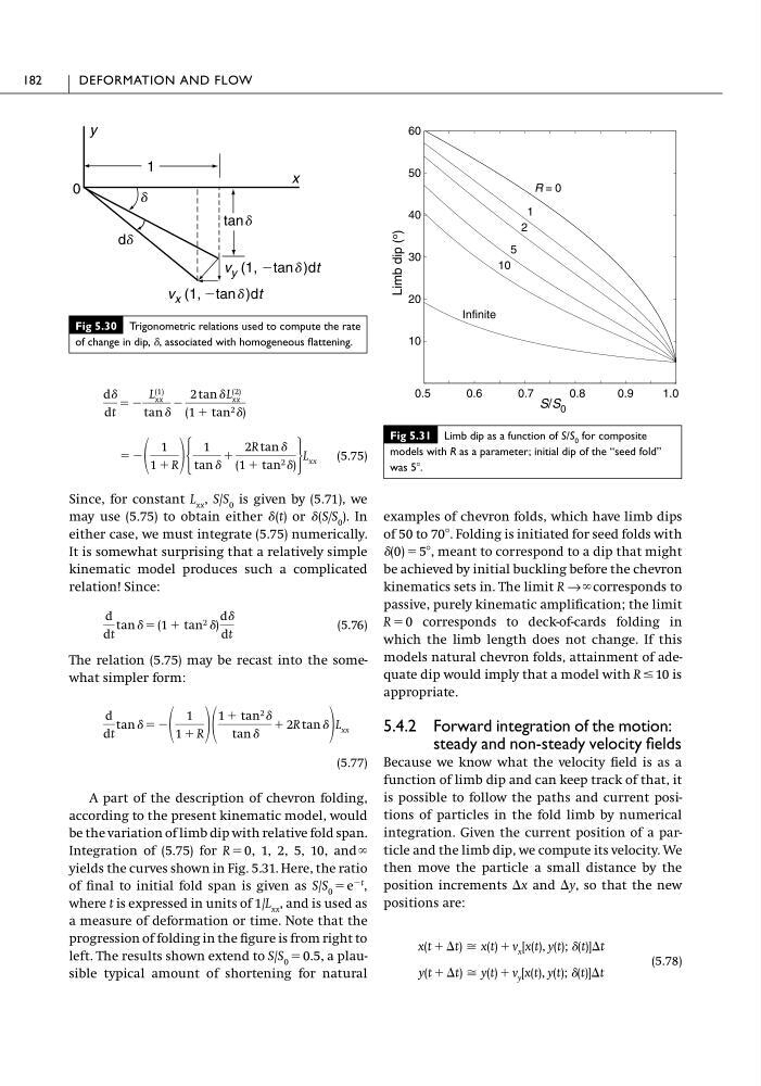
A part of the description of chevron folding,
according to the present kinematic model, would
be the variation of limb dip with relative fold span.
Integration of (5.75) for R ϭ 0, 1, 2, 5, 10, and ϱ
yields the curves shown in Fig. 5.31. Here, the ratio
of final to initial fold span is given as S/S 0 ϭ e
Ϫt ,
where t is expressed in units of 1/L xx , and is used as
a measure of deformation or time. Note that the
progression of folding in the figure is from right to
left. The results shown extend to S/S 0 ϭ 0.5, a plausible typical amount of shortening for natural
d
dt
tan ␦ ϭ Ϫ
1
1 ϩ R
1 ϩ tan 2 ␦
tan ␦
ϩ 2R tan ␦ L xx
d
dt
tan ␦ ϭ (1 ϩ tan 2 ␦)
d␦
dt
ϭ Ϫ
1
1 ϩ R Ά
1
tan ␦
ϩ
2R tan ␦
(1 ϩ tan 2 ␦) ·
L xx
d␦
dt
ϭ Ϫ
L (1)
xx
tan ␦
Ϫ
2 tan ␦ L (2)
xx
(1 ϩ tan 2 ␦)
examples of chevron folds, which have limb dips
of 50 to 70Њ. Folding is initiated for seed folds with
␦(0) ϭ 5Њ, meant to correspond to a dip that might
be achieved by initial buckling before the chevron
kinematics sets in. The limit R → ϱ corresponds to
passive, purely kinematic amplification; the limit
R ϭ 0 corresponds to deck-of-cards folding in
which the limb length does not change. If this
models natural chevron folds, attainment of adequate dip would imply that a model with R Յ 10 is
appropriate.
5.4.2 Forward integration of the motion:
steady and non-steady velocity fields
Because we know what the velocity field is as a
function of limb dip and can keep track of that, it
is possible to follow the paths and current positions of particles in the fold limb by numerical
integration. Given the current position of a particle and the limb dip, we compute its velocity. We
then move the particle a small distance by the
position increments ⌬x and ⌬y, so that the new
positions are:
(5.78)
y(t ϩ ⌬t) Х y(t) ϩ v y [x(t), y(t); ␦(t)]⌬t
x(t ϩ ⌬t) Х x(t) ϩ v x [x(t), y(t); ␦(t)]⌬t
182
DEFORMATION AND FLOW
Fig 5.30 Trigonometric relations used to compute the rate
of change in dip, ␦, associated with homogeneous flattening.
y
x
0
d
dd
v y (1, Ϫtan d)dt
v x (1, Ϫtan d)dt
1
tan d
Fig 5.31 Limb dip as a function of S/S 0 for composite
models with R as a parameter; initial dip of the “seed fold”
was 5Њ.
0.5
0.6
0.7
0.8
0.9
1.0
10
20
30
40
50
60
R = 0
1
10
Infinite
5
2
Limb dip ( o
)
S/S 0
Since, for constant L xx , S/S 0 is given by (5.71), we
may use (5.75) to obtain either ␦(t) or ␦(S/S 0 ). In
either case, we must integrate (5.75) numerically.
It is somewhat surprising that a relatively simple
kinematic model produces such a complicated
relation! Since:
(5.76)
The relation (5.75) may be recast into the somewhat simpler form:
(5.77)
A part of the description of chevron folding,
according to the present kinematic model, would
be the variation of limb dip with relative fold span.
Integration of (5.75) for R ϭ 0, 1, 2, 5, 10, and ϱ
yields the curves shown in Fig. 5.31. Here, the ratio
of final to initial fold span is given as S/S 0 ϭ e
Ϫt ,
where t is expressed in units of 1/L xx , and is used as
a measure of deformation or time. Note that the
progression of folding in the figure is from right to
left. The results shown extend to S/S 0 ϭ 0.5, a plausible typical amount of shortening for natural
d
dt
tan ␦ ϭ Ϫ
1
1 ϩ R
1 ϩ tan 2 ␦
tan ␦
ϩ 2R tan ␦ L xx
d
dt
tan ␦ ϭ (1 ϩ tan 2 ␦)
d␦
dt
ϭ Ϫ
1
1 ϩ R Ά
1
tan ␦
ϩ
2R tan ␦
(1 ϩ tan 2 ␦) ·
L xx
d␦
dt
ϭ Ϫ
L (1)
xx
tan ␦
Ϫ
2 tan ␦ L (2)
xx
(1 ϩ tan 2 ␦)
examples of chevron folds, which have limb dips
of 50 to 70Њ. Folding is initiated for seed folds with
␦(0) ϭ 5Њ, meant to correspond to a dip that might
be achieved by initial buckling before the chevron
kinematics sets in. The limit R → ϱ corresponds to
passive, purely kinematic amplification; the limit
R ϭ 0 corresponds to deck-of-cards folding in
which the limb length does not change. If this
models natural chevron folds, attainment of adequate dip would imply that a model with R Յ 10 is
appropriate.
5.4.2 Forward integration of the motion:
steady and non-steady velocity fields
Because we know what the velocity field is as a
function of limb dip and can keep track of that, it
is possible to follow the paths and current positions of particles in the fold limb by numerical
integration. Given the current position of a particle and the limb dip, we compute its velocity. We
then move the particle a small distance by the
position increments ⌬x and ⌬y, so that the new
positions are:
(5.78)
y(t ϩ ⌬t) Х y(t) ϩ v y [x(t), y(t); ␦(t)]⌬t
x(t ϩ ⌬t) Х x(t) ϩ v x [x(t), y(t); ␦(t)]⌬t
182
DEFORMATION AND FLOW
Fig 5.30 Trigonometric relations used to compute the rate
of change in dip, ␦, associated with homogeneous flattening.
y
x
0
d
dd
v y (1, Ϫtan d)dt
v x (1, Ϫtan d)dt
1
tan d
Fig 5.31 Limb dip as a function of S/S 0 for composite
models with R as a parameter; initial dip of the “seed fold”
was 5Њ.
0.5
0.6
0.7
0.8
0.9
1.0
10
20
30
40
50
60
R = 0
1
10
Infinite
5
2
Limb dip ( o
)
S/S 0