

One might then ask which value of R best simulates
a natural chevron fold in terms of amount of interlayer slip and homogeneous layer deformation on
the fold limb. With the choice of L xx as defining the
rate of the process, we may replace f 1 and f 2 in (5.65)
using (5.69). The combined model is:
(5.70)
v y ϭ ΄
1
1 ϩ R
1
tan ␦
Ϫ tan ␦ x Ϫ y ΅ L xx
v x ϭ L xx x
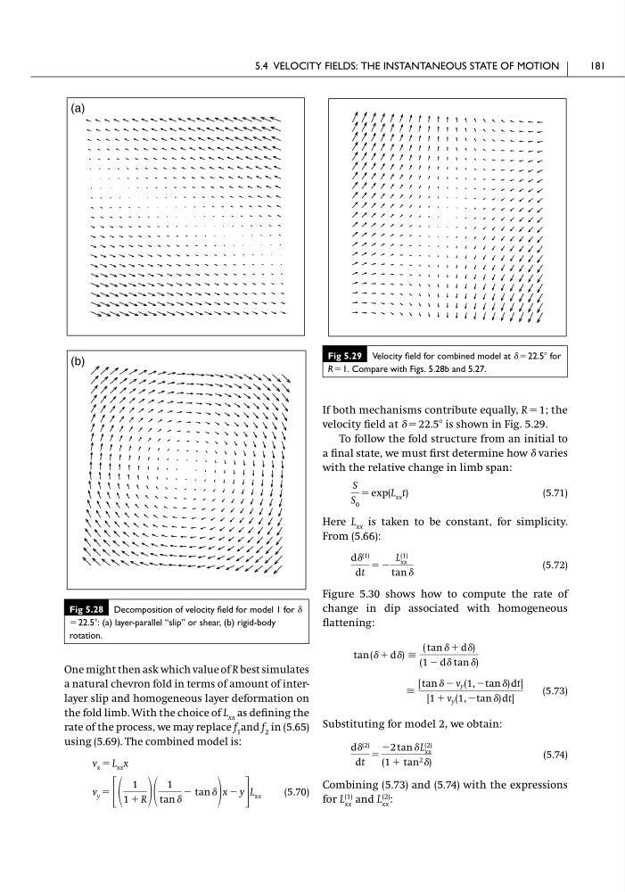
If both mechanisms contribute equally, R ϭ 1; the
velocity field at ␦ ϭ 22.5Њ is shown in Fig. 5.29.
To follow the fold structure from an initial to
a final state, we must first determine how ␦ varies
with the relative change in limb span:
(5.71)
Here L xx is taken to be constant, for simplicity.
From (5.66):
(5.72)
Figure 5.30 shows how to compute the rate of
change in dip associated with homogeneous
flattening:
(5.73)
Substituting for model 2, we obtain:
(5.74)
Combining (5.73) and (5.74) with the expressions
for L xx
(1) and L xx
(2)
:
d␦ (2)
dt
ϭ
Ϫ2 tan ␦ L (2)
xx
(1 ϩ tan 2 ␦)
Х
[ tan ␦ Ϫ v y (1, Ϫ tan ␦) dt]
[1 ϩ v y (1, Ϫ tan ␦) dt]
tan (␦ ϩ d␦) Х
( tan ␦ ϩ d␦)
(1 Ϫ d␦ tan ␦)
d␦ (1)
dt
ϭ Ϫ
L (1)
xx
tan ␦
S
S 0
ϭ exp(L xx t)
5.4 VELOCITY FIELDS: THE INSTANTANEOUS STATE OF MOTION
181
Fig 5.28 Decomposition of velocity field for model 1 for ␦
ϭ 22.5Њ: (a) layer-parallel “slip” or shear, (b) rigid-body
rotation.
(a)
(b)
Fig 5.29 Velocity field for combined model at ␦ϭ22.5Њ for
R ϭ1. Compare with Figs. 5.28b and 5.27.
a natural chevron fold in terms of amount of interlayer slip and homogeneous layer deformation on
the fold limb. With the choice of L xx as defining the
rate of the process, we may replace f 1 and f 2 in (5.65)
using (5.69). The combined model is:
(5.70)
v y ϭ ΄
1
1 ϩ R
1
tan ␦
Ϫ tan ␦ x Ϫ y ΅ L xx
v x ϭ L xx x
If both mechanisms contribute equally, R ϭ 1; the
velocity field at ␦ ϭ 22.5Њ is shown in Fig. 5.29.
To follow the fold structure from an initial to
a final state, we must first determine how ␦ varies
with the relative change in limb span:
(5.71)
Here L xx is taken to be constant, for simplicity.
From (5.66):
(5.72)
Figure 5.30 shows how to compute the rate of
change in dip associated with homogeneous
flattening:
(5.73)
Substituting for model 2, we obtain:
(5.74)
Combining (5.73) and (5.74) with the expressions
for L xx
(1) and L xx
(2)
:
d␦ (2)
dt
ϭ
Ϫ2 tan ␦ L (2)
xx
(1 ϩ tan 2 ␦)
Х
[ tan ␦ Ϫ v y (1, Ϫ tan ␦) dt]
[1 ϩ v y (1, Ϫ tan ␦) dt]
tan (␦ ϩ d␦) Х
( tan ␦ ϩ d␦)
(1 Ϫ d␦ tan ␦)
d␦ (1)
dt
ϭ Ϫ
L (1)
xx
tan ␦
S
S 0
ϭ exp(L xx t)
5.4 VELOCITY FIELDS: THE INSTANTANEOUS STATE OF MOTION
181
Fig 5.28 Decomposition of velocity field for model 1 for ␦
ϭ 22.5Њ: (a) layer-parallel “slip” or shear, (b) rigid-body
rotation.
(a)
(b)
Fig 5.29 Velocity field for combined model at ␦ϭ22.5Њ for
R ϭ1. Compare with Figs. 5.28b and 5.27.