

(5.64)
The shear is expressed by the velocity field
obtained by subtracting (5.64) from (5.63). The
latter looks complicated, but yields a result like
that in Fig. 5.28a for any choice of ␦.
5.4.1 Combined model for chevron
folding
We now formulate a kinematic model that combines the De Sitter model, model 1, and the homogeneous flattening model, model 2. The velocity
field for the combined model is formed by summing
the two velocity fields in some proportion:
(5.65)
The fractions f 1 and f 2 might be taken to be functions of time or limb dip. This model is ad hoc,
since we have advanced no physical principles
that would allow us to fix f 1 and f 2 . We present
these models to illustrate results that might
approximately simulate the development of
chevron folds and to provide some experience in
thinking about kinematics and deformation.
The fact that the velocity field of the De Sitter
model (model 1) is expressed in terms of the rate
of change in dip, d␦/dt, creates difficulty. We
might use the dip itself as a time-like variable, and
assign some arbitrary constant value to d␦/dt.
However, the dip is also changed by homogeneous
flattening (model 2). As one way of proceeding, we
express the progress of folding by means of the
rate of change in the span of the limb, normalized
by the span itself. For model 1:
(5.66)
For model 2:
(5.67)
΄
1
S
dS
dt ΅
(2)
ϭ L (2)
xx
ϭ
1
S L (1)
xx S ϭ Ϫ tan ␦
d␦
dt
΄
1
S
dS
dt ΅
(1)
ϭ
1
S v (1)
x (S, 0)
f 1 ϩ f 2 ϭ 1
v y ϭ f 1 v (1)
y ϩ f 2 v (2)
y
v x ϭ f 1 v (1)
x ϩ f 2 v (2)
x
(v y ) rotation
d␦
dt
Ϫ1
ϭ x
(v x ) rotation
d␦
dt
Ϫ1
ϭ Ϫy
The total relative rate of change of S, as might have
been anticipated, is:
(5.68)
A simple combined model is one in which the
individual contributions are in constant ratio:
(5.69)
L (1)
xx ϭ
L xx
1 ϩ R
, L (2)
xx ϭ
RL xx
1 ϩ R
, R ϭ
L (2)
xx
L (1)
xx
1
S
dS
dt
ϭ L (1)
xx ϩ L (2)
xx ϭ L xx
180
DEFORMATION AND FLOW
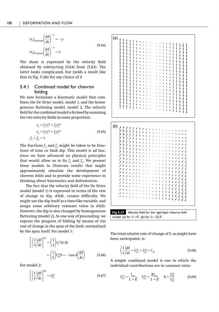
Fig 5.27 Velocity field for the rigid layer chevron fold
model: (a) for ␦ϭ0Њ, (b) for ␦ϭ22.5Њ.
(a)
(b)
The shear is expressed by the velocity field
obtained by subtracting (5.64) from (5.63). The
latter looks complicated, but yields a result like
that in Fig. 5.28a for any choice of ␦.
5.4.1 Combined model for chevron
folding
We now formulate a kinematic model that combines the De Sitter model, model 1, and the homogeneous flattening model, model 2. The velocity
field for the combined model is formed by summing
the two velocity fields in some proportion:
(5.65)
The fractions f 1 and f 2 might be taken to be functions of time or limb dip. This model is ad hoc,
since we have advanced no physical principles
that would allow us to fix f 1 and f 2 . We present
these models to illustrate results that might
approximately simulate the development of
chevron folds and to provide some experience in
thinking about kinematics and deformation.
The fact that the velocity field of the De Sitter
model (model 1) is expressed in terms of the rate
of change in dip, d␦/dt, creates difficulty. We
might use the dip itself as a time-like variable, and
assign some arbitrary constant value to d␦/dt.
However, the dip is also changed by homogeneous
flattening (model 2). As one way of proceeding, we
express the progress of folding by means of the
rate of change in the span of the limb, normalized
by the span itself. For model 1:
(5.66)
For model 2:
(5.67)
΄
1
S
dS
dt ΅
(2)
ϭ L (2)
xx
ϭ
1
S L (1)
xx S ϭ Ϫ tan ␦
d␦
dt
΄
1
S
dS
dt ΅
(1)
ϭ
1
S v (1)
x (S, 0)
f 1 ϩ f 2 ϭ 1
v y ϭ f 1 v (1)
y ϩ f 2 v (2)
y
v x ϭ f 1 v (1)
x ϩ f 2 v (2)
x
(v y ) rotation
d␦
dt
Ϫ1
ϭ x
(v x ) rotation
d␦
dt
Ϫ1
ϭ Ϫy
The total relative rate of change of S, as might have
been anticipated, is:
(5.68)
A simple combined model is one in which the
individual contributions are in constant ratio:
(5.69)
L (1)
xx ϭ
L xx
1 ϩ R
, L (2)
xx ϭ
RL xx
1 ϩ R
, R ϭ
L (2)
xx
L (1)
xx
1
S
dS
dt
ϭ L (1)
xx ϩ L (2)
xx ϭ L xx
180
DEFORMATION AND FLOW
Fig 5.27 Velocity field for the rigid layer chevron fold
model: (a) for ␦ϭ0Њ, (b) for ␦ϭ22.5Њ.
(a)
(b)