

time. In the simplest case they are constant.
Integration then yields:
(5.58)
The condition of constant area requires F yy (t) ϭ
1/F xx (t), or, from (5.58):
(5.59)
Indeed, constant area requires (5.59) whatever the
time variation of these quantities. The time frame
during which structures form is an interesting
topic brought up by considerations of velocity. It
is significant to questions such as that of the connection between folding and gold mineralization
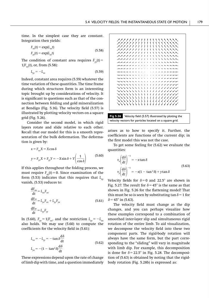
at Bendigo (Fig. 5.16). The velocity field (5.57) is
illustrated by plotting velocity vectors on a square
grid (Fig. 5.26).
Consider the second model, in which rigid
layers rotate and slide relative to each other.
Recall that our model for this is a smooth representation of the bulk deformation. The deformation is given by:
(5.60)
If this applies throughout the folding process, we
must require F xy (t) ϭ 0. Since examination of the
form (5.53) indicates that this requires that L xy
vanish, (5.53) reduces to:
(5.61)
In (5.60), F yy ϭ 1/F xx , and the restriction L yy ϭϪL xx
also holds. We may use (5.60) to compute the
coefficients for the velocity field in (5.61):
(5.62)
These expressions depend upon the rate of change
of limb dip with time, and a question immediately
L yx ϭ Ϫ(1 Ϫ tan 2 ␦)
d␦
dt
L xx ϭ ϪL yy ϭ Ϫ tan ␦
d␦
dt
dFyy
dt
ϭ L yy F yy
dFyx
dt
ϭ L yx F xx ϩ L yy F yx
dF xx
dt
ϭ L xx F xx
y ϭ F yx X ϩ F yy Y ϭ ϪX sin ␦ ϩ Y
1
cos ␦
x ϭ F xx X ϭ X cos ␦
L yy ϭ ϪL xx
F yy (t) ϭ exp(L yy t)
F xx (t) ϭ exp(L xx t)
arises as to how to specify it. Further, the
coefficients are functions of the current dip; in
the first model this was not the case.
To get some feeling for (5.62) we evaluate the
quantities:
(5.63)
Velocity fields for ␦ ϭ 0 and 22.5Њ are shown in
Fig. 5.27. The result for ␦ ϭ 45Њ is the same as that
shown in Fig. 5.26 for the flattening model! That
this must be so is seen by substituting tan ␦ ϭ 1 for
␦ ϭ 45Њ in (5.63).
The velocity field must change as the dip
changes, and you can perhaps visualize how
these examples correspond to a combination of
smoothed inter-layer slip and simultaneous rigid
rotation of the entire limb. To aid visualization,
we decompose the velocity field into these two
component parts. The rigid-body rotation will
always have the same form, but the part corresponding to the “sliding” will vary in magnitude
with limb dip. For example, this decomposition
is done for ␦ ϭ 22.5Њ in Fig. 5.28. The decomposition of (5.63) is obtained by noting that the rigidbody rotation (Fig. 5.28b) is expressed as:
v y
d␦
dt
Ϫ1
ϭ Ϫx(1 Ϫ tan 2 ␦) ϩ y tan ␦
v x
d␦
dt
Ϫ1
ϭ Ϫx tan ␦
5.4 VELOCITY FIELDS: THE INSTANTANEOUS STATE OF MOTION
179
Fig 5.26 Velocity field (5.57) illustrated by plotting the
velocity vectors for particles located on a square grid.
Integration then yields:
(5.58)
The condition of constant area requires F yy (t) ϭ
1/F xx (t), or, from (5.58):
(5.59)
Indeed, constant area requires (5.59) whatever the
time variation of these quantities. The time frame
during which structures form is an interesting
topic brought up by considerations of velocity. It
is significant to questions such as that of the connection between folding and gold mineralization
at Bendigo (Fig. 5.16). The velocity field (5.57) is
illustrated by plotting velocity vectors on a square
grid (Fig. 5.26).
Consider the second model, in which rigid
layers rotate and slide relative to each other.
Recall that our model for this is a smooth representation of the bulk deformation. The deformation is given by:
(5.60)
If this applies throughout the folding process, we
must require F xy (t) ϭ 0. Since examination of the
form (5.53) indicates that this requires that L xy
vanish, (5.53) reduces to:
(5.61)
In (5.60), F yy ϭ 1/F xx , and the restriction L yy ϭϪL xx
also holds. We may use (5.60) to compute the
coefficients for the velocity field in (5.61):
(5.62)
These expressions depend upon the rate of change
of limb dip with time, and a question immediately
L yx ϭ Ϫ(1 Ϫ tan 2 ␦)
d␦
dt
L xx ϭ ϪL yy ϭ Ϫ tan ␦
d␦
dt
dFyy
dt
ϭ L yy F yy
dFyx
dt
ϭ L yx F xx ϩ L yy F yx
dF xx
dt
ϭ L xx F xx
y ϭ F yx X ϩ F yy Y ϭ ϪX sin ␦ ϩ Y
1
cos ␦
x ϭ F xx X ϭ X cos ␦
L yy ϭ ϪL xx
F yy (t) ϭ exp(L yy t)
F xx (t) ϭ exp(L xx t)
arises as to how to specify it. Further, the
coefficients are functions of the current dip; in
the first model this was not the case.
To get some feeling for (5.62) we evaluate the
quantities:
(5.63)
Velocity fields for ␦ ϭ 0 and 22.5Њ are shown in
Fig. 5.27. The result for ␦ ϭ 45Њ is the same as that
shown in Fig. 5.26 for the flattening model! That
this must be so is seen by substituting tan ␦ ϭ 1 for
␦ ϭ 45Њ in (5.63).
The velocity field must change as the dip
changes, and you can perhaps visualize how
these examples correspond to a combination of
smoothed inter-layer slip and simultaneous rigid
rotation of the entire limb. To aid visualization,
we decompose the velocity field into these two
component parts. The rigid-body rotation will
always have the same form, but the part corresponding to the “sliding” will vary in magnitude
with limb dip. For example, this decomposition
is done for ␦ ϭ 22.5Њ in Fig. 5.28. The decomposition of (5.63) is obtained by noting that the rigidbody rotation (Fig. 5.28b) is expressed as:
v y
d␦
dt
Ϫ1
ϭ Ϫx(1 Ϫ tan 2 ␦) ϩ y tan ␦
v x
d␦
dt
Ϫ1
ϭ Ϫx tan ␦
5.4 VELOCITY FIELDS: THE INSTANTANEOUS STATE OF MOTION
179
Fig 5.26 Velocity field (5.57) illustrated by plotting the
velocity vectors for particles located on a square grid.