

Here, x and y are used to describe the current coordinates of some particle in the body, but they are
also used to describe position in space. The use of
these quantities to describe current position of
particular particles and position within the body
creates no problem. For example, the velocity at a
particular position is an attribute of the particle
currently occupying this position. The mathematical description of the variation in velocity with
position may be smoothly varying. While we may
formally evaluate the function elsewhere than
within the body, e.g. within a hole in the body, it
is clear that the values of quantities there have no
physical significance.
The velocity field within the body at a particular instant of time will depend upon the physical
state of the body, its properties, and the forces
applied to it. Thus, rather than the current state
of deformation, with reference to some initial
configuration, it is this that we must look to if we
want to understand the process producing the
structure of interest. We will examine this relationship in this textbook. An example given in
this chapter is that of the Stokes solution.
However, we also want to know how the history of
the instantaneous state of motion, or the velocity
field, gives rise to the current or final structure;
and within the limited context of kinematics that
is something we may accomplish in this chapter.
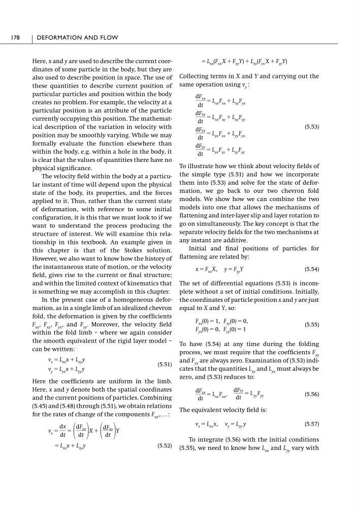
In the present case of a homogeneous deformation, as in a single limb of an idealized chevron
fold, the deformation is given by the coefficients
F xx , F xy , F yx , and F yy . Moreover, the velocity field
within the fold limb – where we again consider
the smooth equivalent of the rigid layer model –
can be written:
(5.51)
Here the coefficients are uniform in the limb.
Here, x and y denote both the spatial coordinates
and the current positions of particles. Combining
(5.45) and (5.48) through (5.51), we obtain relations
for the rates of change of the components F xx ,. . . :
(5.52)
ϭ L xx x ϩ L xy y
v x ϭ
dx
dt
ϭ
dF xx
dt X ϩ
dF xy
dt Y
v y ϭ L yx x ϩ L yy y
v x ϭ L xx x ϩ L xy y
Collecting terms in X and Y and carrying out the
same operation using v y :
(5.53)
To illustrate how we think about velocity fields of
the simple type (5.51) and how we incorporate
them into (5.53) and solve for the state of deformation, we go back to our two chevron fold
models. We show how we can combine the two
models into one that allows the mechanisms of
flattening and inter-layer slip and layer rotation to
go on simultaneously. The key concept is that the
separate velocity fields for the two mechanisms at
any instant are additive.
Initial and final positions of particles for
flattening are related by:
(5.54)
The set of differential equations (5.53) is incomplete without a set of initial conditions. Initially,
the coordinates of particle position x and y are just
equal to X and Y, so:
(5.55)
To have (5.54) at any time during the folding
process, we must require that the coefficients F xy
and F yx are always zero. Examination of (5.53) indicates that the quantities L xy and L yx must always be
zero, and (5.53) reduces to:
(5.56)
The equivalent velocity field is:
(5.57)
To integrate (5.56) with the initial conditions
(5.55), we need to know how L xx and L yy vary with
v x ϭ L xx x, v y ϭ L yy y
dF xx
dt
ϭ L xx F xx ,
dFyy
dt
ϭ L yy F yy
F yx (0) ϭ 0, F yy (0) ϭ 1
F xx (0) ϭ 1, F xy (0) ϭ 0,
x ϭ F xx X, y ϭ F yy Y
dFyy
dt
ϭ L yx F xy ϩ L yy F yy
dFyx
dt
ϭ L yx F xx ϩ L yy F yx
dFxy
dt
ϭ L xx F xy ϩ L xy F yy
dF xx
dt
ϭ L xx F xx ϩ L xy F yx
ϭ L xx (F xx X ϩ F xy Y) ϩ L xy (F yx X ϩ F yy Y)
178
DEFORMATION AND FLOW
also used to describe position in space. The use of
these quantities to describe current position of
particular particles and position within the body
creates no problem. For example, the velocity at a
particular position is an attribute of the particle
currently occupying this position. The mathematical description of the variation in velocity with
position may be smoothly varying. While we may
formally evaluate the function elsewhere than
within the body, e.g. within a hole in the body, it
is clear that the values of quantities there have no
physical significance.
The velocity field within the body at a particular instant of time will depend upon the physical
state of the body, its properties, and the forces
applied to it. Thus, rather than the current state
of deformation, with reference to some initial
configuration, it is this that we must look to if we
want to understand the process producing the
structure of interest. We will examine this relationship in this textbook. An example given in
this chapter is that of the Stokes solution.
However, we also want to know how the history of
the instantaneous state of motion, or the velocity
field, gives rise to the current or final structure;
and within the limited context of kinematics that
is something we may accomplish in this chapter.
In the present case of a homogeneous deformation, as in a single limb of an idealized chevron
fold, the deformation is given by the coefficients
F xx , F xy , F yx , and F yy . Moreover, the velocity field
within the fold limb – where we again consider
the smooth equivalent of the rigid layer model –
can be written:
(5.51)
Here the coefficients are uniform in the limb.
Here, x and y denote both the spatial coordinates
and the current positions of particles. Combining
(5.45) and (5.48) through (5.51), we obtain relations
for the rates of change of the components F xx ,. . . :
(5.52)
ϭ L xx x ϩ L xy y
v x ϭ
dx
dt
ϭ
dF xx
dt X ϩ
dF xy
dt Y
v y ϭ L yx x ϩ L yy y
v x ϭ L xx x ϩ L xy y
Collecting terms in X and Y and carrying out the
same operation using v y :
(5.53)
To illustrate how we think about velocity fields of
the simple type (5.51) and how we incorporate
them into (5.53) and solve for the state of deformation, we go back to our two chevron fold
models. We show how we can combine the two
models into one that allows the mechanisms of
flattening and inter-layer slip and layer rotation to
go on simultaneously. The key concept is that the
separate velocity fields for the two mechanisms at
any instant are additive.
Initial and final positions of particles for
flattening are related by:
(5.54)
The set of differential equations (5.53) is incomplete without a set of initial conditions. Initially,
the coordinates of particle position x and y are just
equal to X and Y, so:
(5.55)
To have (5.54) at any time during the folding
process, we must require that the coefficients F xy
and F yx are always zero. Examination of (5.53) indicates that the quantities L xy and L yx must always be
zero, and (5.53) reduces to:
(5.56)
The equivalent velocity field is:
(5.57)
To integrate (5.56) with the initial conditions
(5.55), we need to know how L xx and L yy vary with
v x ϭ L xx x, v y ϭ L yy y
dF xx
dt
ϭ L xx F xx ,
dFyy
dt
ϭ L yy F yy
F yx (0) ϭ 0, F yy (0) ϭ 1
F xx (0) ϭ 1, F xy (0) ϭ 0,
x ϭ F xx X, y ϭ F yy Y
dFyy
dt
ϭ L yx F xy ϩ L yy F yy
dFyx
dt
ϭ L yx F xx ϩ L yy F yx
dFxy
dt
ϭ L xx F xy ϩ L xy F yy
dF xx
dt
ϭ L xx F xx ϩ L xy F yx
ϭ L xx (F xx X ϩ F xy Y) ϩ L xy (F yx X ϩ F yy Y)
178
DEFORMATION AND FLOW