

Models of the sub-surface fault geometry are
needed as well as the mechanical properties
(seismic wave velocities) of the rock from the
fault to the location of the seismographs.
The use of interferometric synthetic aperture
radar (InSAR) for the detection of ground displacements associated with earthquakes was
highlighted in articles appearing in the early
1990s (Massonnet et al., 1993; Prescott, 1993;
Zebker et al., 1994). The radar signal is transmitted
from a satellite to the ground surface where it is
reflected back to the satellite and recorded as a
set of pixels making up an image of the surface.
Knowledge of the travel time and speed of the
signal provide the information necessary to calculate the range, or distance, from the satellite
to each reflective site on the surface. If the same
region is imaged at two different times, for
example before and after the earthquake, the difference between the two images can be used to calculate the component of the surface displacement
directed toward the satellite. The resulting image
(Fig. 1.2e), called an interferogram, is similar to a
contour map of the displacement component on
which the white and black bands (called fringes)
are the contours. The fault segments are shown as
fine white lines superimposed on this image. By
invoking a model (usually based on elasticity
theory) for the location and geometry of the fault
segments and the mechanical behavior of the
rock mass, one may use this displacement distribution on Earth’s surface to calculate the
corresponding slip distribution on the fault. The
abundance of data provides considerable constraint on the unknown slip distribution below
Earth’s surface and very exciting avenues for new
research on faulting.
It should be obvious from this discussion that
the different disciplines contribute information
that is based on different observations in different
locations and over different length and time
scales. Yet scientists from all three disciplines are
studying the same physical phenomenon, faulting, and they are using the same tools to build
their models, namely elasticity theory. In this
textbook we focus on the geological data and the
models that are used to relate measurements
of slip to fault behavior. On the other hand each
discipline is providing important pieces of the
puzzle, so structural geologists should be aware of
the concepts and contributions from geophysics
and geodesy to the study of faulting. In addition
important insights are attained from studying the
effects of faulting on the geomorphology of the
landscape (Arrowsmith et al., 1996; Arrowsmith
et al., 1998). The most comprehensive view of
faults and the faulting process will come from an
integration of all these data and that integration
will be most effective in the context of building
well-constrained models.
1.1.2 Conceptual and mechanical models
for the 1979 earthquake rupture
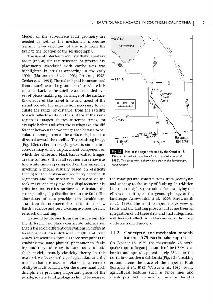
On October 15, 1979, the magnitude 6.5 earthquake rupture began just south of the US–Mexico
border and spread approximately 35 km to the
north into southern California (Fig. 1.3), breaking
ground along the trace of the Imperial Fault
(Johnson et al., 1982; Wosser et al., 1982). Many
agricultural features such as fence lines and
canals provided markers to measure the slip
1.1 EARTHQUAKE HAZARDS IN SOUTHERN CALIFORNIA
5
SALTON SEA
111
78
111
86
111
8
UN ITE D STA TES
ME XIC O
I m p e r ia l
Brawley
Fault
zone
10
0
km
E A S T
H IG H L IN E
33 o 15'
33 o 15'
32
o 45'
F a u lt
CA NA L
Epicenter
10/15/79
115 o 30'
115
o 45'
Fig 1.3 Map of the region affected by the October 15,
1979, earthquake in southern California (Wosser et al.,
1982). The epicenter is shown as a star in the lower righthand corner.
needed as well as the mechanical properties
(seismic wave velocities) of the rock from the
fault to the location of the seismographs.
The use of interferometric synthetic aperture
radar (InSAR) for the detection of ground displacements associated with earthquakes was
highlighted in articles appearing in the early
1990s (Massonnet et al., 1993; Prescott, 1993;
Zebker et al., 1994). The radar signal is transmitted
from a satellite to the ground surface where it is
reflected back to the satellite and recorded as a
set of pixels making up an image of the surface.
Knowledge of the travel time and speed of the
signal provide the information necessary to calculate the range, or distance, from the satellite
to each reflective site on the surface. If the same
region is imaged at two different times, for
example before and after the earthquake, the difference between the two images can be used to calculate the component of the surface displacement
directed toward the satellite. The resulting image
(Fig. 1.2e), called an interferogram, is similar to a
contour map of the displacement component on
which the white and black bands (called fringes)
are the contours. The fault segments are shown as
fine white lines superimposed on this image. By
invoking a model (usually based on elasticity
theory) for the location and geometry of the fault
segments and the mechanical behavior of the
rock mass, one may use this displacement distribution on Earth’s surface to calculate the
corresponding slip distribution on the fault. The
abundance of data provides considerable constraint on the unknown slip distribution below
Earth’s surface and very exciting avenues for new
research on faulting.
It should be obvious from this discussion that
the different disciplines contribute information
that is based on different observations in different
locations and over different length and time
scales. Yet scientists from all three disciplines are
studying the same physical phenomenon, faulting, and they are using the same tools to build
their models, namely elasticity theory. In this
textbook we focus on the geological data and the
models that are used to relate measurements
of slip to fault behavior. On the other hand each
discipline is providing important pieces of the
puzzle, so structural geologists should be aware of
the concepts and contributions from geophysics
and geodesy to the study of faulting. In addition
important insights are attained from studying the
effects of faulting on the geomorphology of the
landscape (Arrowsmith et al., 1996; Arrowsmith
et al., 1998). The most comprehensive view of
faults and the faulting process will come from an
integration of all these data and that integration
will be most effective in the context of building
well-constrained models.
1.1.2 Conceptual and mechanical models
for the 1979 earthquake rupture
On October 15, 1979, the magnitude 6.5 earthquake rupture began just south of the US–Mexico
border and spread approximately 35 km to the
north into southern California (Fig. 1.3), breaking
ground along the trace of the Imperial Fault
(Johnson et al., 1982; Wosser et al., 1982). Many
agricultural features such as fence lines and
canals provided markers to measure the slip
1.1 EARTHQUAKE HAZARDS IN SOUTHERN CALIFORNIA
5
SALTON SEA
111
78
111
86
111
8
UN ITE D STA TES
ME XIC O
I m p e r ia l
Brawley
Fault
zone
10
0
km
E A S T
H IG H L IN E
33 o 15'
33 o 15'
32
o 45'
F a u lt
CA NA L
Epicenter
10/15/79
115 o 30'
115
o 45'
Fig 1.3 Map of the region affected by the October 15,
1979, earthquake in southern California (Wosser et al.,
1982). The epicenter is shown as a star in the lower righthand corner.