

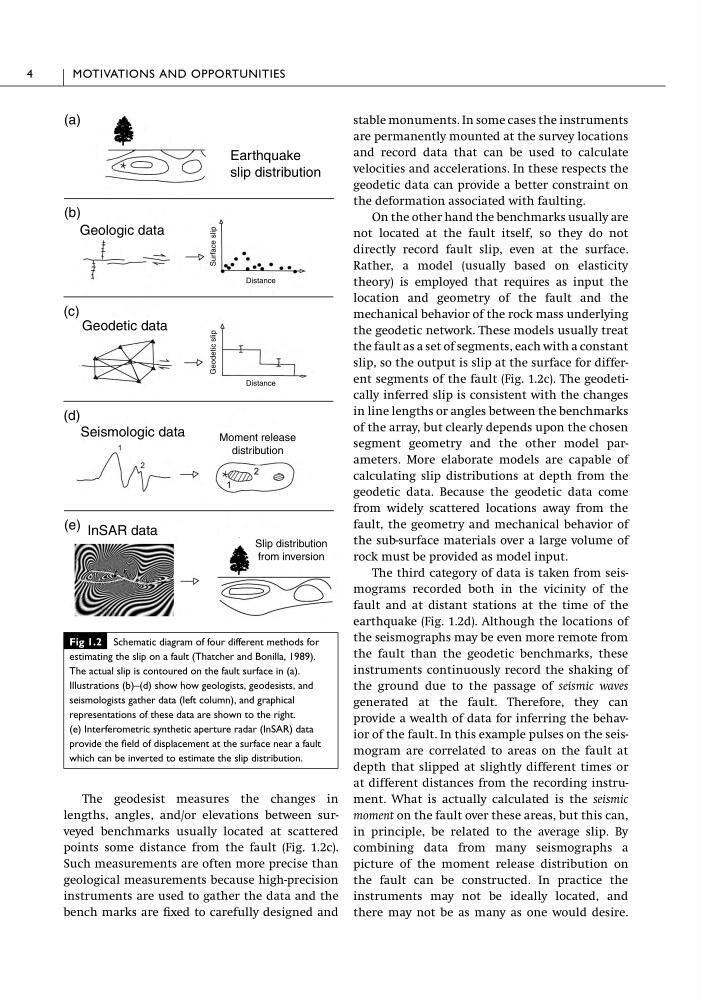
The geodesist measures the changes in
lengths, angles, and/or elevations between surveyed benchmarks usually located at scattered
points some distance from the fault (Fig. 1.2c).
Such measurements are often more precise than
geological measurements because high-precision
instruments are used to gather the data and the
bench marks are fixed to carefully designed and
stable monuments. In some cases the instruments
are permanently mounted at the survey locations
and record data that can be used to calculate
velocities and accelerations. In these respects the
geodetic data can provide a better constraint on
the deformation associated with faulting.
On the other hand the benchmarks usually are
not located at the fault itself, so they do not
directly record fault slip, even at the surface.
Rather, a model (usually based on elasticity
theory) is employed that requires as input the
location and geometry of the fault and the
mechanical behavior of the rock mass underlying
the geodetic network. These models usually treat
the fault as a set of segments, each with a constant
slip, so the output is slip at the surface for different segments of the fault (Fig. 1.2c). The geodetically inferred slip is consistent with the changes
in line lengths or angles between the benchmarks
of the array, but clearly depends upon the chosen
segment geometry and the other model parameters. More elaborate models are capable of
calculating slip distributions at depth from the
geodetic data. Because the geodetic data come
from widely scattered locations away from the
fault, the geometry and mechanical behavior of
the sub-surface materials over a large volume of
rock must be provided as model input.
The third category of data is taken from seismograms recorded both in the vicinity of the
fault and at distant stations at the time of the
earthquake (Fig. 1.2d). Although the locations of
the seismographs may be even more remote from
the fault than the geodetic benchmarks, these
instruments continuously record the shaking of
the ground due to the passage of seismic waves
generated at the fault. Therefore, they can
provide a wealth of data for inferring the behavior of the fault. In this example pulses on the seismogram are correlated to areas on the fault at
depth that slipped at slightly different times or
at different distances from the recording instrument. What is actually calculated is the seismic
moment on the fault over these areas, but this can,
in principle, be related to the average slip. By
combining data from many seismographs a
picture of the moment release distribution on
the fault can be constructed. In practice the
instruments may not be ideally located, and
there may not be as many as one would desire.
4
MOTIVATIONS AND OPPORTUNITIES
(a)
(b)
(c)
(d)
(e)
Earthquake
slip distribution
Geologic data
Geodetic data
Seismologic data
InSAR data
Moment release
distribution
Slip distribution
from inversion
Surface slip
Geodetic slip
Distance
Distance
Fig 1.2 Schematic diagram of four different methods for
estimating the slip on a fault (Thatcher and Bonilla, 1989).
The actual slip is contoured on the fault surface in (a).
Illustrations (b)–(d) show how geologists, geodesists, and
seismologists gather data (left column), and graphical
representations of these data are shown to the right.
(e) Interferometric synthetic aperture radar (InSAR) data
provide the field of displacement at the surface near a fault
which can be inverted to estimate the slip distribution.
lengths, angles, and/or elevations between surveyed benchmarks usually located at scattered
points some distance from the fault (Fig. 1.2c).
Such measurements are often more precise than
geological measurements because high-precision
instruments are used to gather the data and the
bench marks are fixed to carefully designed and
stable monuments. In some cases the instruments
are permanently mounted at the survey locations
and record data that can be used to calculate
velocities and accelerations. In these respects the
geodetic data can provide a better constraint on
the deformation associated with faulting.
On the other hand the benchmarks usually are
not located at the fault itself, so they do not
directly record fault slip, even at the surface.
Rather, a model (usually based on elasticity
theory) is employed that requires as input the
location and geometry of the fault and the
mechanical behavior of the rock mass underlying
the geodetic network. These models usually treat
the fault as a set of segments, each with a constant
slip, so the output is slip at the surface for different segments of the fault (Fig. 1.2c). The geodetically inferred slip is consistent with the changes
in line lengths or angles between the benchmarks
of the array, but clearly depends upon the chosen
segment geometry and the other model parameters. More elaborate models are capable of
calculating slip distributions at depth from the
geodetic data. Because the geodetic data come
from widely scattered locations away from the
fault, the geometry and mechanical behavior of
the sub-surface materials over a large volume of
rock must be provided as model input.
The third category of data is taken from seismograms recorded both in the vicinity of the
fault and at distant stations at the time of the
earthquake (Fig. 1.2d). Although the locations of
the seismographs may be even more remote from
the fault than the geodetic benchmarks, these
instruments continuously record the shaking of
the ground due to the passage of seismic waves
generated at the fault. Therefore, they can
provide a wealth of data for inferring the behavior of the fault. In this example pulses on the seismogram are correlated to areas on the fault at
depth that slipped at slightly different times or
at different distances from the recording instrument. What is actually calculated is the seismic
moment on the fault over these areas, but this can,
in principle, be related to the average slip. By
combining data from many seismographs a
picture of the moment release distribution on
the fault can be constructed. In practice the
instruments may not be ideally located, and
there may not be as many as one would desire.
4
MOTIVATIONS AND OPPORTUNITIES
(a)
(b)
(c)
(d)
(e)
Earthquake
slip distribution
Geologic data
Geodetic data
Seismologic data
InSAR data
Moment release
distribution
Slip distribution
from inversion
Surface slip
Geodetic slip
Distance
Distance
Fig 1.2 Schematic diagram of four different methods for
estimating the slip on a fault (Thatcher and Bonilla, 1989).
The actual slip is contoured on the fault surface in (a).
Illustrations (b)–(d) show how geologists, geodesists, and
seismologists gather data (left column), and graphical
representations of these data are shown to the right.
(e) Interferometric synthetic aperture radar (InSAR) data
provide the field of displacement at the surface near a fault
which can be inverted to estimate the slip distribution.