

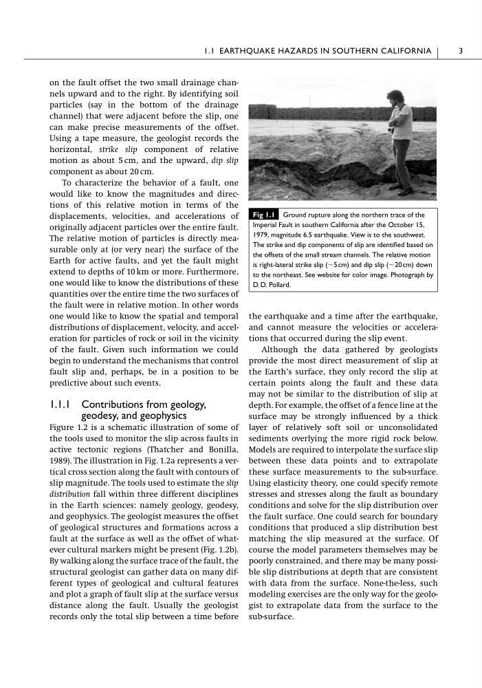
on the fault offset the two small drainage channels upward and to the right. By identifying soil
particles (say in the bottom of the drainage
channel) that were adjacent before the slip, one
can make precise measurements of the offset.
Using a tape measure, the geologist records the
horizontal, strike slip component of relative
motion as about 5 cm, and the upward, dip slip
component as about 20 cm.
To characterize the behavior of a fault, one
would like to know the magnitudes and directions of this relative motion in terms of the
displacements, velocities, and accelerations of
originally adjacent particles over the entire fault.
The relative motion of particles is directly measurable only at (or very near) the surface of the
Earth for active faults, and yet the fault might
extend to depths of 10 km or more. Furthermore,
one would like to know the distributions of these
quantities over the entire time the two surfaces of
the fault were in relative motion. In other words
one would like to know the spatial and temporal
distributions of displacement, velocity, and acceleration for particles of rock or soil in the vicinity
of the fault. Given such information we could
begin to understand the mechanisms that control
fault slip and, perhaps, be in a position to be
predictive about such events.
1.1.1 Contributions from geology,
geodesy, and geophysics
Figure 1.2 is a schematic illustration of some of
the tools used to monitor the slip across faults in
active tectonic regions (Thatcher and Bonilla,
1989). The illustration in Fig. 1.2a represents a vertical cross section along the fault with contours of
slip magnitude. The tools used to estimate the slip
distribution fall within three different disciplines
in the Earth sciences: namely geology, geodesy,
and geophysics. The geologist measures the offset
of geological structures and formations across a
fault at the surface as well as the offset of whatever cultural markers might be present (Fig. 1.2b).
By walking along the surface trace of the fault, the
structural geologist can gather data on many different types of geological and cultural features
and plot a graph of fault slip at the surface versus
distance along the fault. Usually the geologist
records only the total slip between a time before
the earthquake and a time after the earthquake,
and cannot measure the velocities or accelerations that occurred during the slip event.
Although the data gathered by geologists
provide the most direct measurement of slip at
the Earth’s surface, they only record the slip at
certain points along the fault and these data
may not be similar to the distribution of slip at
depth. For example, the offset of a fence line at the
surface may be strongly influenced by a thick
layer of relatively soft soil or unconsolidated
sediments overlying the more rigid rock below.
Models are required to interpolate the surface slip
between these data points and to extrapolate
these surface measurements to the sub-surface.
Using elasticity theory, one could specify remote
stresses and stresses along the fault as boundary
conditions and solve for the slip distribution over
the fault surface. One could search for boundary
conditions that produced a slip distribution best
matching the slip measured at the surface. Of
course the model parameters themselves may be
poorly constrained, and there may be many possible slip distributions at depth that are consistent
with data from the surface. None-the-less, such
modeling exercises are the only way for the geologist to extrapolate data from the surface to the
sub-surface.
1.1 EARTHQUAKE HAZARDS IN SOUTHERN CALIFORNIA
3
Fig 1.1 Ground rupture along the northern trace of the
Imperial Fault in southern California after the October 15,
1979, magnitude 6.5 earthquake. View is to the southwest.
The strike and dip components of slip are identified based on
the offsets of the small stream channels. The relative motion
is right-lateral strike slip (ϳ5cm) and dip slip (ϳ20cm) down
to the northeast. See website for color image. Photograph by
D. D. Pollard.
particles (say in the bottom of the drainage
channel) that were adjacent before the slip, one
can make precise measurements of the offset.
Using a tape measure, the geologist records the
horizontal, strike slip component of relative
motion as about 5 cm, and the upward, dip slip
component as about 20 cm.
To characterize the behavior of a fault, one
would like to know the magnitudes and directions of this relative motion in terms of the
displacements, velocities, and accelerations of
originally adjacent particles over the entire fault.
The relative motion of particles is directly measurable only at (or very near) the surface of the
Earth for active faults, and yet the fault might
extend to depths of 10 km or more. Furthermore,
one would like to know the distributions of these
quantities over the entire time the two surfaces of
the fault were in relative motion. In other words
one would like to know the spatial and temporal
distributions of displacement, velocity, and acceleration for particles of rock or soil in the vicinity
of the fault. Given such information we could
begin to understand the mechanisms that control
fault slip and, perhaps, be in a position to be
predictive about such events.
1.1.1 Contributions from geology,
geodesy, and geophysics
Figure 1.2 is a schematic illustration of some of
the tools used to monitor the slip across faults in
active tectonic regions (Thatcher and Bonilla,
1989). The illustration in Fig. 1.2a represents a vertical cross section along the fault with contours of
slip magnitude. The tools used to estimate the slip
distribution fall within three different disciplines
in the Earth sciences: namely geology, geodesy,
and geophysics. The geologist measures the offset
of geological structures and formations across a
fault at the surface as well as the offset of whatever cultural markers might be present (Fig. 1.2b).
By walking along the surface trace of the fault, the
structural geologist can gather data on many different types of geological and cultural features
and plot a graph of fault slip at the surface versus
distance along the fault. Usually the geologist
records only the total slip between a time before
the earthquake and a time after the earthquake,
and cannot measure the velocities or accelerations that occurred during the slip event.
Although the data gathered by geologists
provide the most direct measurement of slip at
the Earth’s surface, they only record the slip at
certain points along the fault and these data
may not be similar to the distribution of slip at
depth. For example, the offset of a fence line at the
surface may be strongly influenced by a thick
layer of relatively soft soil or unconsolidated
sediments overlying the more rigid rock below.
Models are required to interpolate the surface slip
between these data points and to extrapolate
these surface measurements to the sub-surface.
Using elasticity theory, one could specify remote
stresses and stresses along the fault as boundary
conditions and solve for the slip distribution over
the fault surface. One could search for boundary
conditions that produced a slip distribution best
matching the slip measured at the surface. Of
course the model parameters themselves may be
poorly constrained, and there may be many possible slip distributions at depth that are consistent
with data from the surface. None-the-less, such
modeling exercises are the only way for the geologist to extrapolate data from the surface to the
sub-surface.
1.1 EARTHQUAKE HAZARDS IN SOUTHERN CALIFORNIA
3
Fig 1.1 Ground rupture along the northern trace of the
Imperial Fault in southern California after the October 15,
1979, magnitude 6.5 earthquake. View is to the southwest.
The strike and dip components of slip are identified based on
the offsets of the small stream channels. The relative motion
is right-lateral strike slip (ϳ5cm) and dip slip (ϳ20cm) down
to the northeast. See website for color image. Photograph by
D. D. Pollard.