

fold limbs with localized bending or breaking of
the layers in the narrow hinges. Accordingly, we
introduce another model for fold formation in
which layers do not behave as rigid bodies. We
begin with the limiting case in which inter-layer
slip is excluded.
Start with the configuration shown in Fig.
5.20, which corresponds with perfect chevron
folds of low limb dip. As above, consider a functional relationship that describes the final position of any particle in the body in terms of its
initial position. We choose the simple relationship:
(5.39)
Here F xx and F yy are constants. The initial and final
fold forms are two-dimensional cylindrical forms
with generator or axis parallel to the z-axis.
First consider what happens to a rectangular
element of area in the (x, y)-plane whose initial
corners are the points (0, 0), (0, X), (X, Y ), and (0, Y ).
Its area is XY. In the deformed state, the element
remains a rectangle, with corners at (0, 0), (0,x), (x,
y), and (0, y) and area:
(5.40)
Thus, by choosing F yy ϭ 1/F xx in (5.39) we prescribe
that the cross-sectional area of the body, or any
part of it, remains the same. Referring to a broad
range of structure cross sections, structural geologists refer to this circumstance as one in which
area is conserved. Keep in mind that conservation of
area is NOT a law of nature, such as conservation of
mass. Does the De Sitter model conserve area?
Application of the transformation (5.39) with
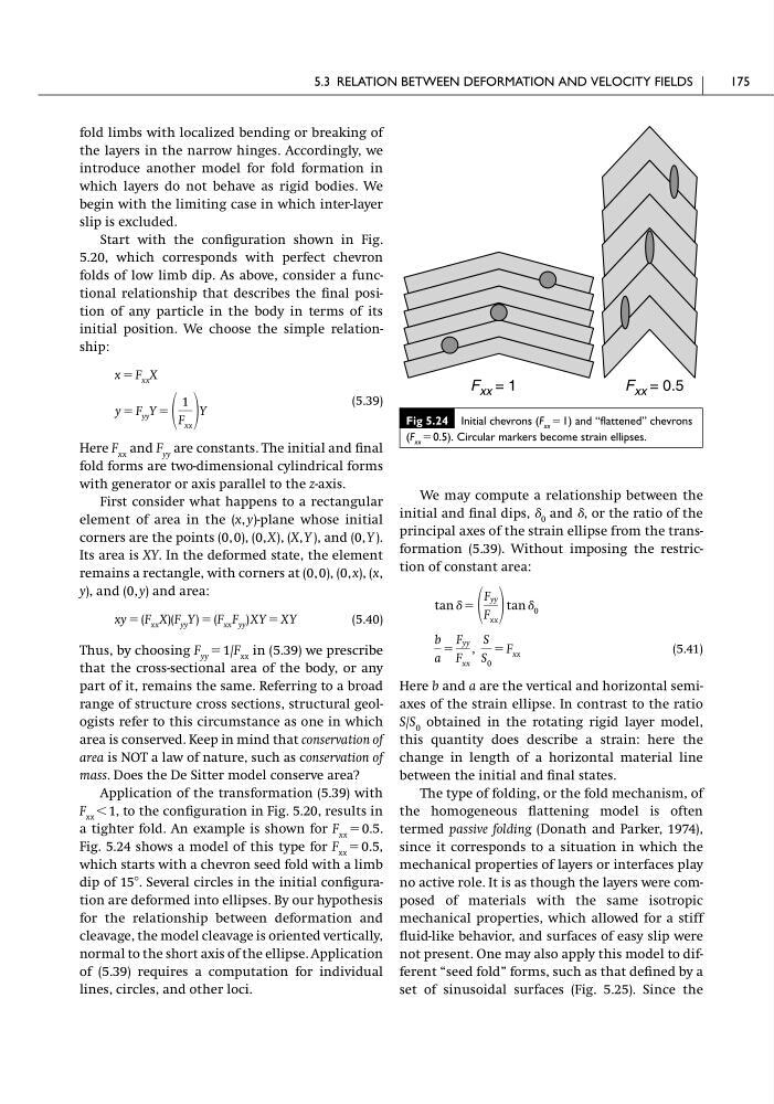
F xx Ͻ 1, to the configuration in Fig. 5.20, results in
a tighter fold. An example is shown for F xx ϭ 0.5.
Fig. 5.24 shows a model of this type for F xx ϭ 0.5,
which starts with a chevron seed fold with a limb
dip of 15Њ. Several circles in the initial configuration are deformed into ellipses. By our hypothesis
for the relationship between deformation and
cleavage, the model cleavage is oriented vertically,
normal to the short axis of the ellipse. Application
of (5.39) requires a computation for individual
lines, circles, and other loci.
xy ϭ (F xx X)(F yy Y) ϭ (F xx F yy ) XY ϭ XY
y ϭ F yy Y ϭ
1
F xx
Y
x ϭ F xx X
We may compute a relationship between the
initial and final dips, ␦ 0 and ␦, or the ratio of the
principal axes of the strain ellipse from the transformation (5.39). Without imposing the restriction of constant area:
(5.41)
Here b and a are the vertical and horizontal semiaxes of the strain ellipse. In contrast to the ratio
S/S 0 obtained in the rotating rigid layer model,
this quantity does describe a strain: here the
change in length of a horizontal material line
between the initial and final states.
The type of folding, or the fold mechanism, of
the homogeneous flattening model is often
termed passive folding (Donath and Parker, 1974),
since it corresponds to a situation in which the
mechanical properties of layers or interfaces play
no active role. It is as though the layers were composed of materials with the same isotropic
mechanical properties, which allowed for a stiff
fluid-like behavior, and surfaces of easy slip were
not present. One may also apply this model to different “seed fold” forms, such as that defined by a
set of sinusoidal surfaces (Fig. 5.25). Since the
b
a
ϭ
F yy
F xx
,
S
S 0
ϭ F xx
tan ␦ ϭ
F yy
F xx
tan ␦ 0
5.3 RELATION BETWEEN DEFORMATION AND VELOCITY FIELDS
175
Fig 5.24 Initial chevrons (F xx ϭ1) and “flattened” chevrons
(F xx ϭ0.5). Circular markers become strain ellipses.
F xx = 1
F xx = 0.5
the layers in the narrow hinges. Accordingly, we
introduce another model for fold formation in
which layers do not behave as rigid bodies. We
begin with the limiting case in which inter-layer
slip is excluded.
Start with the configuration shown in Fig.
5.20, which corresponds with perfect chevron
folds of low limb dip. As above, consider a functional relationship that describes the final position of any particle in the body in terms of its
initial position. We choose the simple relationship:
(5.39)
Here F xx and F yy are constants. The initial and final
fold forms are two-dimensional cylindrical forms
with generator or axis parallel to the z-axis.
First consider what happens to a rectangular
element of area in the (x, y)-plane whose initial
corners are the points (0, 0), (0, X), (X, Y ), and (0, Y ).
Its area is XY. In the deformed state, the element
remains a rectangle, with corners at (0, 0), (0,x), (x,
y), and (0, y) and area:
(5.40)
Thus, by choosing F yy ϭ 1/F xx in (5.39) we prescribe
that the cross-sectional area of the body, or any
part of it, remains the same. Referring to a broad
range of structure cross sections, structural geologists refer to this circumstance as one in which
area is conserved. Keep in mind that conservation of
area is NOT a law of nature, such as conservation of
mass. Does the De Sitter model conserve area?
Application of the transformation (5.39) with
F xx Ͻ 1, to the configuration in Fig. 5.20, results in
a tighter fold. An example is shown for F xx ϭ 0.5.
Fig. 5.24 shows a model of this type for F xx ϭ 0.5,
which starts with a chevron seed fold with a limb
dip of 15Њ. Several circles in the initial configuration are deformed into ellipses. By our hypothesis
for the relationship between deformation and
cleavage, the model cleavage is oriented vertically,
normal to the short axis of the ellipse. Application
of (5.39) requires a computation for individual
lines, circles, and other loci.
xy ϭ (F xx X)(F yy Y) ϭ (F xx F yy ) XY ϭ XY
y ϭ F yy Y ϭ
1
F xx
Y
x ϭ F xx X
We may compute a relationship between the
initial and final dips, ␦ 0 and ␦, or the ratio of the
principal axes of the strain ellipse from the transformation (5.39). Without imposing the restriction of constant area:
(5.41)
Here b and a are the vertical and horizontal semiaxes of the strain ellipse. In contrast to the ratio
S/S 0 obtained in the rotating rigid layer model,
this quantity does describe a strain: here the
change in length of a horizontal material line
between the initial and final states.
The type of folding, or the fold mechanism, of
the homogeneous flattening model is often
termed passive folding (Donath and Parker, 1974),
since it corresponds to a situation in which the
mechanical properties of layers or interfaces play
no active role. It is as though the layers were composed of materials with the same isotropic
mechanical properties, which allowed for a stiff
fluid-like behavior, and surfaces of easy slip were
not present. One may also apply this model to different “seed fold” forms, such as that defined by a
set of sinusoidal surfaces (Fig. 5.25). Since the
b
a
ϭ
F yy
F xx
,
S
S 0
ϭ F xx
tan ␦ ϭ
F yy
F xx
tan ␦ 0
5.3 RELATION BETWEEN DEFORMATION AND VELOCITY FIELDS
175
Fig 5.24 Initial chevrons (F xx ϭ1) and “flattened” chevrons
(F xx ϭ0.5). Circular markers become strain ellipses.
F xx = 1
F xx = 0.5