

variety is endless we should begin to think about
what folds in rock actually look like and how they
might have formed as constrained by the laws of
physics and explicitly defined material properties.
These considerations will be taken up in later
chapters – for now we are limited to geometry and
kinematics.
5.3.5 Inter-layer slip and homogeneous
flattening
Since both the rigid layer slip model and the
homogeneous deformation models of geometry
and kinematics are quite simple, we may combine
them to obtain a chevron fold model that shows
both characteristic features: inter-layer slip and
cleavage. One simple procedure for combining the
models is to first apply one model, or mechanism,
to achieve a fold form from an initial configuration, and then apply the other mechanism to the
structure produced to achieve the final fold. This
mirrors the two-part procedure of first slipping
the layers in the fold limb, and then subjecting
the whole to a rigid-body rotation, or vice versa
(Fig. 5.21b). For example, beginning with the De
Sitter model, the fold is obtained by first applying
the transformation:
x (1) ϭ X cos ␦ (1)
(5.42)
Here, we have assumed that the initial dip is vanishingly small. To obtain the final form, the transformation (5.39) is applied to (5.42):
(5.43)
Substituting from (5.42) we have:
(5.44)
Notice that the forms of the coefficients are:
(5.45)
In these equations the coefficients are:
(5.46)
The quantities F xx
(1) ,. . . , are given in (5.42). Here,
and throughout this section, we describe the De
Sitter model in terms of its continuous medium
approximation. We can appreciate that the algebraic complexity of such a description increases
rapidly, although the operation itself is straightforward. Imagine applying each of the two mechanisms alternately over many steps!
The final dip ␦ is:
(5.47)
The final limb dip ␦ may be measured, and if
strain markers allowed b/a to be determined, (5.47)
provides an estimate of the limb dip at which
layer-parallel slip ceased – according to the model!
Because the circular sections are simply
rotated during the layer-slip stage, and no slip
occurs during the second stage, cleavage in the
fold will be vertical. If we observe a chevron fold
tan ␦ ϭ
1
F (2)
xx
2
tan ␦ (1) ϭ
b
a tan ␦ (1)
F yy ϭ F (2)
yx F (1)
xy ϩ F (2)
yy F (1)
yy
F yx ϭ F (2)
yx F (1)
xx ϩ F (2)
yy F (1)
yx
F xy ϭ F (2)
xx F (1)
xy ϩ F (2)
xy F (1)
yy
F xx ϭ F (2)
xx F (1)
xx ϩ F (2)
xy F (1)
yx
y ϭ F yx X ϩ F yy Y
x ϭ F xx X ϩ F xy Y
y ϭ
1
F (2)
xx
΄ ϪX sin ␦ (1) ϩ
1
cos ␦ (1) Y ΅
x ϭ (F (2)
xx cos ␦ (1) ) X
y ϭ
1
F (2)
xx
y (1)
x ϭ F (2)
xx x (1)
y (1) ϭ ϪX sin ␦ (1) ϩ Y
1
cos ␦ (1)
176
DEFORMATION AND FLOW
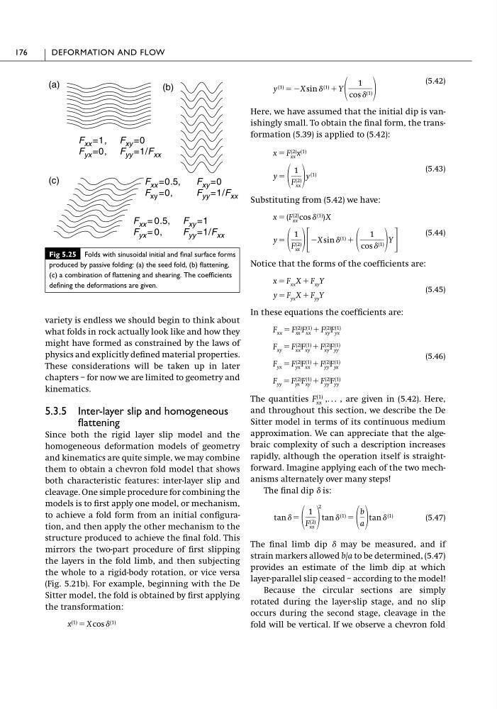
Fig 5.25 Folds with sinusoidal initial and final surface forms
produced by passive folding: (a) the seed fold, (b) flattening,
(c) a combination of flattening and shearing. The coefficients
defining the deformations are given.
F xx = 0.5, F xy =1
F yx = 0,
F yy =1/F xx
F xx =0.5,
F xy =0
F xy =0,
F yy =1/F xx
F xx =1, F xy =0
F yx =0, F yy =1/F xx
(a)
(b)
(c)
what folds in rock actually look like and how they
might have formed as constrained by the laws of
physics and explicitly defined material properties.
These considerations will be taken up in later
chapters – for now we are limited to geometry and
kinematics.
5.3.5 Inter-layer slip and homogeneous
flattening
Since both the rigid layer slip model and the
homogeneous deformation models of geometry
and kinematics are quite simple, we may combine
them to obtain a chevron fold model that shows
both characteristic features: inter-layer slip and
cleavage. One simple procedure for combining the
models is to first apply one model, or mechanism,
to achieve a fold form from an initial configuration, and then apply the other mechanism to the
structure produced to achieve the final fold. This
mirrors the two-part procedure of first slipping
the layers in the fold limb, and then subjecting
the whole to a rigid-body rotation, or vice versa
(Fig. 5.21b). For example, beginning with the De
Sitter model, the fold is obtained by first applying
the transformation:
x (1) ϭ X cos ␦ (1)
(5.42)
Here, we have assumed that the initial dip is vanishingly small. To obtain the final form, the transformation (5.39) is applied to (5.42):
(5.43)
Substituting from (5.42) we have:
(5.44)
Notice that the forms of the coefficients are:
(5.45)
In these equations the coefficients are:
(5.46)
The quantities F xx
(1) ,. . . , are given in (5.42). Here,
and throughout this section, we describe the De
Sitter model in terms of its continuous medium
approximation. We can appreciate that the algebraic complexity of such a description increases
rapidly, although the operation itself is straightforward. Imagine applying each of the two mechanisms alternately over many steps!
The final dip ␦ is:
(5.47)
The final limb dip ␦ may be measured, and if
strain markers allowed b/a to be determined, (5.47)
provides an estimate of the limb dip at which
layer-parallel slip ceased – according to the model!
Because the circular sections are simply
rotated during the layer-slip stage, and no slip
occurs during the second stage, cleavage in the
fold will be vertical. If we observe a chevron fold
tan ␦ ϭ
1
F (2)
xx
2
tan ␦ (1) ϭ
b
a tan ␦ (1)
F yy ϭ F (2)
yx F (1)
xy ϩ F (2)
yy F (1)
yy
F yx ϭ F (2)
yx F (1)
xx ϩ F (2)
yy F (1)
yx
F xy ϭ F (2)
xx F (1)
xy ϩ F (2)
xy F (1)
yy
F xx ϭ F (2)
xx F (1)
xx ϩ F (2)
xy F (1)
yx
y ϭ F yx X ϩ F yy Y
x ϭ F xx X ϩ F xy Y
y ϭ
1
F (2)
xx
΄ ϪX sin ␦ (1) ϩ
1
cos ␦ (1) Y ΅
x ϭ (F (2)
xx cos ␦ (1) ) X
y ϭ
1
F (2)
xx
y (1)
x ϭ F (2)
xx x (1)
y (1) ϭ ϪX sin ␦ (1) ϩ Y
1
cos ␦ (1)
176
DEFORMATION AND FLOW
Fig 5.25 Folds with sinusoidal initial and final surface forms
produced by passive folding: (a) the seed fold, (b) flattening,
(c) a combination of flattening and shearing. The coefficients
defining the deformations are given.
F xx = 0.5, F xy =1
F yx = 0,
F yy =1/F xx
F xx =0.5,
F xy =0
F xy =0,
F yy =1/F xx
F xx =1, F xy =0
F yx =0, F yy =1/F xx
(a)
(b)
(c)