

Since the layers are rigid in the model, a material
line element within an individual layer does not
change its length and no such element undergoes
strain. It will be useful to formulate a concept of
bulk strain for the fold limb as a whole.
A rock mass cut by numerous faults may
undergo a bulk strain for a set of displacements on
the faults. The present model affords a simple
example of such a situation, the “faults” being the
layer-parallel or bed-parallel slip surfaces. Since
rock bodies may deform by the relative motion of
many approximately rigid elements, down to individual grains or grain fragments, this concept of
bulk strain has many applications. In the present
case, the slip across each interface is:
(5.30)
Here ␦ 0 is the initial dip of the “seed fold.” The
negative sign is adopted because the fold limb of
Fig. 5.21a may be produced from the unfolded
configuration by first sliding each layer above the
pinned layer at the origin to the left by this
amount and then rotating the whole limb by –␦.
The physics convention is that a positive rotation
is counterclockwise (Fig. 5.21b).
We now seek a description of the two-dimensional deformation that corresponds to the De
Sitter chevron fold model:
(5.31)
The description (5.31) will be developed using the
fixed coordinate axes of Fig. 5.21 to which initial
and final coordinates will be referred. Since the
layers rotate about axes parallel to z and particles
move in cross-sectional planes of constant z we
have z ϭ Z. The particle at the origin remains
there:
(5.32)
If (5.31) is to be specified for all particles in the
body for the rigid layer model, called the De Sitter
model, they must be specified for each and every
layer, since the slip between layers means that
these functions cannot be continuous functions
of initial position. This could be done in a compact
form by identifying the pair of functions for each
y(0, 0) ϭ 0
x(0, 0) ϭ 0
y ϭ y(X, Y )
x ϭ x(X, Y )
u ϭ ϪH( tan ␦ Ϫ tan ␦ 0 )
layer with the Y-coordinate of its center point. For
the nth layer upward, this would be nH, and downward, ϪnH. To avoid such complexity, at least initially, let us agree to find the functions (5.31) that
apply only to the particles located on the centerlines of the layers. For these particles, the functions may be written as though the particle
displacements were continuous. We thus obtain a
description of the bulk deformation of the fold
limb.
We write down continuous functions that
capture exactly the initial and final positions of
the particles on the mid-planes. These are most
easily found by consulting Fig. 5.21b and combining the results for the two steps. Coordinates of
the intermediate positions are:
(5.33)
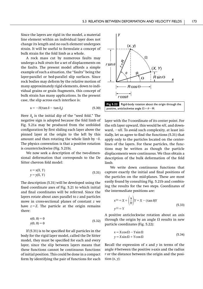
A positive anticlockwise rotation about an axis
through the origin by an angle ⍀ results in new
particle coordinates (Fig. 5.22):
(5.34)
Recall the expression of x and y in terms of the
angle between the positive x-axis and the radius
r or the distance between the origin and the position (x, y):
y ϭ X sin ⍀ ϩ Y cos ⍀
x ϭ X cos ⍀ Ϫ Y sin ⍀
y (1) ϭ Y
x (1) ϭ X ϩ
u
H Y ϭ X Ϫ ( tan ␦)Y
5.3 RELATION BETWEEN DEFORMATION AND VELOCITY FIELDS
173
Fig 5.22 Rigid-body rotation about the origin through the
positive, anticlockwise angle ⍀ϭϪ⌰.
y
(x, y)
⍀
r = R
u
R
r cosu
x
(X, Y)
R cos ⍜
R sin ⍜
⍜
r sin u
line element within an individual layer does not
change its length and no such element undergoes
strain. It will be useful to formulate a concept of
bulk strain for the fold limb as a whole.
A rock mass cut by numerous faults may
undergo a bulk strain for a set of displacements on
the faults. The present model affords a simple
example of such a situation, the “faults” being the
layer-parallel or bed-parallel slip surfaces. Since
rock bodies may deform by the relative motion of
many approximately rigid elements, down to individual grains or grain fragments, this concept of
bulk strain has many applications. In the present
case, the slip across each interface is:
(5.30)
Here ␦ 0 is the initial dip of the “seed fold.” The
negative sign is adopted because the fold limb of
Fig. 5.21a may be produced from the unfolded
configuration by first sliding each layer above the
pinned layer at the origin to the left by this
amount and then rotating the whole limb by –␦.
The physics convention is that a positive rotation
is counterclockwise (Fig. 5.21b).
We now seek a description of the two-dimensional deformation that corresponds to the De
Sitter chevron fold model:
(5.31)
The description (5.31) will be developed using the
fixed coordinate axes of Fig. 5.21 to which initial
and final coordinates will be referred. Since the
layers rotate about axes parallel to z and particles
move in cross-sectional planes of constant z we
have z ϭ Z. The particle at the origin remains
there:
(5.32)
If (5.31) is to be specified for all particles in the
body for the rigid layer model, called the De Sitter
model, they must be specified for each and every
layer, since the slip between layers means that
these functions cannot be continuous functions
of initial position. This could be done in a compact
form by identifying the pair of functions for each
y(0, 0) ϭ 0
x(0, 0) ϭ 0
y ϭ y(X, Y )
x ϭ x(X, Y )
u ϭ ϪH( tan ␦ Ϫ tan ␦ 0 )
layer with the Y-coordinate of its center point. For
the nth layer upward, this would be nH, and downward, ϪnH. To avoid such complexity, at least initially, let us agree to find the functions (5.31) that
apply only to the particles located on the centerlines of the layers. For these particles, the functions may be written as though the particle
displacements were continuous. We thus obtain a
description of the bulk deformation of the fold
limb.
We write down continuous functions that
capture exactly the initial and final positions of
the particles on the mid-planes. These are most
easily found by consulting Fig. 5.21b and combining the results for the two steps. Coordinates of
the intermediate positions are:
(5.33)
A positive anticlockwise rotation about an axis
through the origin by an angle ⍀ results in new
particle coordinates (Fig. 5.22):
(5.34)
Recall the expression of x and y in terms of the
angle between the positive x-axis and the radius
r or the distance between the origin and the position (x, y):
y ϭ X sin ⍀ ϩ Y cos ⍀
x ϭ X cos ⍀ Ϫ Y sin ⍀
y (1) ϭ Y
x (1) ϭ X ϩ
u
H Y ϭ X Ϫ ( tan ␦)Y
5.3 RELATION BETWEEN DEFORMATION AND VELOCITY FIELDS
173
Fig 5.22 Rigid-body rotation about the origin through the
positive, anticlockwise angle ⍀ϭϪ⌰.
y
(x, y)
⍀
r = R
u
R
r cosu
x
(X, Y)
R cos ⍜
R sin ⍜
⍜
r sin u