

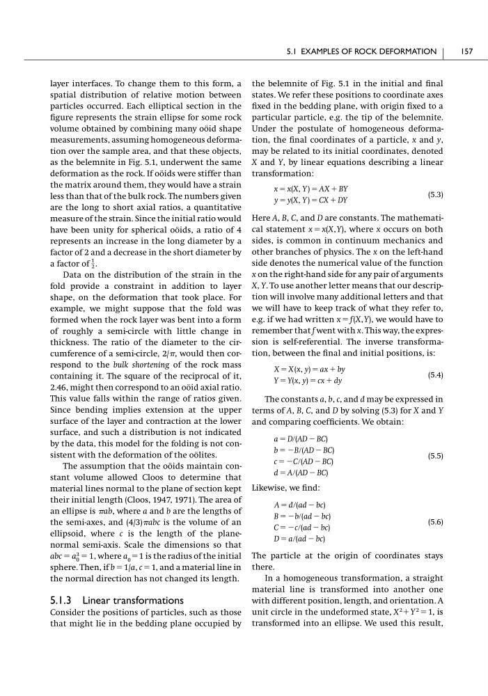
layer interfaces. To change them to this form, a
spatial distribution of relative motion between
particles occurred. Each elliptical section in the
figure represents the strain ellipse for some rock
volume obtained by combining many oöid shape
measurements, assuming homogeneous deformation over the sample area, and that these objects,
as the belemnite in Fig. 5.1, underwent the same
deformation as the rock. If oöids were stiffer than
the matrix around them, they would have a strain
less than that of the bulk rock. The numbers given
are the long to short axial ratios, a quantitative
measure of the strain. Since the initial ratio would
have been unity for spherical oöids, a ratio of 4
represents an increase in the long diameter by a
factor of 2 and a decrease in the short diameter by
a factor of .
Data on the distribution of the strain in the
fold provide a constraint in addition to layer
shape, on the deformation that took place. For
example, we might suppose that the fold was
formed when the rock layer was bent into a form
of roughly a semi-circle with little change in
thickness. The ratio of the diameter to the circumference of a semi-circle, 2/, would then correspond to the bulk shortening of the rock mass
containing it. The square of the reciprocal of it,
2.46, might then correspond to an oöid axial ratio.
This value falls within the range of ratios given.
Since bending implies extension at the upper
surface of the layer and contraction at the lower
surface, and such a distribution is not indicated
by the data, this model for the folding is not consistent with the deformation of the oölites.
The assumption that the oöids maintain constant volume allowed Cloos to determine that
material lines normal to the plane of section kept
their initial length (Cloos, 1947, 1971). The area of
an ellipse is ab, where a and b are the lengths of
the semi-axes, and (4/3)abc is the volume of an
ellipsoid, where c is the length of the planenormal semi-axis. Scale the dimensions so that
, where a 0 ϭ1 is the radius of the initial
sphere. Then, if b ϭ 1/a, c ϭ 1, and a material line in
the normal direction has not changed its length.
5.1.3 Linear transformations
Consider the positions of particles, such as those
that might lie in the bedding plane occupied by
abc ϭ a 3
0 ϭ 1
1
2
the belemnite of Fig. 5.1 in the initial and final
states. We refer these positions to coordinate axes
fixed in the bedding plane, with origin fixed to a
particular particle, e.g. the tip of the belemnite.
Under the postulate of homogeneous deformation, the final coordinates of a particle, x and y,
may be related to its initial coordinates, denoted
X and Y, by linear equations describing a linear
transformation:
(5.3)
Here A, B, C, and D are constants. The mathematical statement x ϭ x(X, Y), where x occurs on both
sides, is common in continuum mechanics and
other branches of physics. The x on the left-hand
side denotes the numerical value of the function
x on the right-hand side for any pair of arguments
X, Y. To use another letter means that our description will involve many additional letters and that
we will have to keep track of what they refer to,
e.g. if we had written x ϭ f(X, Y), we would have to
remember that f went with x. This way, the expression is self-referential. The inverse transformation, between the final and initial positions, is:
(5.4)
The constants a, b, c, and d may be expressed in
terms of A, B, C, and D by solving (5.3) for X and Y
and comparing coefficients. We obtain:
(5.5)
Likewise, we find:
(5.6)
The particle at the origin of coordinates stays
there.
In a homogeneous transformation, a straight
material line is transformed into another one
with different position, length, and orientation. A
unit circle in the undeformed state, X
2 ϩY
2 ϭ 1, is
transformed into an ellipse. We used this result,
D ϭ aր(ad Ϫ bc)
C ϭ Ϫcր(ad Ϫ bc)
B ϭ Ϫbր(ad Ϫ bc)
A ϭ dր(ad Ϫ bc)
d ϭ Aր(AD Ϫ BC)
c ϭ ϪCր(AD Ϫ BC)
b ϭ ϪBր(AD Ϫ BC)
a ϭ Dր(AD Ϫ BC)
Y ϭ Y(x, y) ϭ cx ϩ dy
X ϭ X (x, y) ϭ ax ϩ by
y ϭ y(X, Y ) ϭ CX ϩ DY
x ϭ x(X, Y ) ϭ AX ϩ BY
5.1 EXAMPLES OF ROCK DEFORMATION
157
spatial distribution of relative motion between
particles occurred. Each elliptical section in the
figure represents the strain ellipse for some rock
volume obtained by combining many oöid shape
measurements, assuming homogeneous deformation over the sample area, and that these objects,
as the belemnite in Fig. 5.1, underwent the same
deformation as the rock. If oöids were stiffer than
the matrix around them, they would have a strain
less than that of the bulk rock. The numbers given
are the long to short axial ratios, a quantitative
measure of the strain. Since the initial ratio would
have been unity for spherical oöids, a ratio of 4
represents an increase in the long diameter by a
factor of 2 and a decrease in the short diameter by
a factor of .
Data on the distribution of the strain in the
fold provide a constraint in addition to layer
shape, on the deformation that took place. For
example, we might suppose that the fold was
formed when the rock layer was bent into a form
of roughly a semi-circle with little change in
thickness. The ratio of the diameter to the circumference of a semi-circle, 2/, would then correspond to the bulk shortening of the rock mass
containing it. The square of the reciprocal of it,
2.46, might then correspond to an oöid axial ratio.
This value falls within the range of ratios given.
Since bending implies extension at the upper
surface of the layer and contraction at the lower
surface, and such a distribution is not indicated
by the data, this model for the folding is not consistent with the deformation of the oölites.
The assumption that the oöids maintain constant volume allowed Cloos to determine that
material lines normal to the plane of section kept
their initial length (Cloos, 1947, 1971). The area of
an ellipse is ab, where a and b are the lengths of
the semi-axes, and (4/3)abc is the volume of an
ellipsoid, where c is the length of the planenormal semi-axis. Scale the dimensions so that
, where a 0 ϭ1 is the radius of the initial
sphere. Then, if b ϭ 1/a, c ϭ 1, and a material line in
the normal direction has not changed its length.
5.1.3 Linear transformations
Consider the positions of particles, such as those
that might lie in the bedding plane occupied by
abc ϭ a 3
0 ϭ 1
1
2
the belemnite of Fig. 5.1 in the initial and final
states. We refer these positions to coordinate axes
fixed in the bedding plane, with origin fixed to a
particular particle, e.g. the tip of the belemnite.
Under the postulate of homogeneous deformation, the final coordinates of a particle, x and y,
may be related to its initial coordinates, denoted
X and Y, by linear equations describing a linear
transformation:
(5.3)
Here A, B, C, and D are constants. The mathematical statement x ϭ x(X, Y), where x occurs on both
sides, is common in continuum mechanics and
other branches of physics. The x on the left-hand
side denotes the numerical value of the function
x on the right-hand side for any pair of arguments
X, Y. To use another letter means that our description will involve many additional letters and that
we will have to keep track of what they refer to,
e.g. if we had written x ϭ f(X, Y), we would have to
remember that f went with x. This way, the expression is self-referential. The inverse transformation, between the final and initial positions, is:
(5.4)
The constants a, b, c, and d may be expressed in
terms of A, B, C, and D by solving (5.3) for X and Y
and comparing coefficients. We obtain:
(5.5)
Likewise, we find:
(5.6)
The particle at the origin of coordinates stays
there.
In a homogeneous transformation, a straight
material line is transformed into another one
with different position, length, and orientation. A
unit circle in the undeformed state, X
2 ϩY
2 ϭ 1, is
transformed into an ellipse. We used this result,
D ϭ aր(ad Ϫ bc)
C ϭ Ϫcր(ad Ϫ bc)
B ϭ Ϫbր(ad Ϫ bc)
A ϭ dր(ad Ϫ bc)
d ϭ Aր(AD Ϫ BC)
c ϭ ϪCր(AD Ϫ BC)
b ϭ ϪBր(AD Ϫ BC)
a ϭ Dր(AD Ϫ BC)
Y ϭ Y(x, y) ϭ cx ϩ dy
X ϭ X (x, y) ϭ ax ϩ by
y ϭ y(X, Y ) ϭ CX ϩ DY
x ϭ x(X, Y ) ϭ AX ϩ BY
5.1 EXAMPLES OF ROCK DEFORMATION
157