

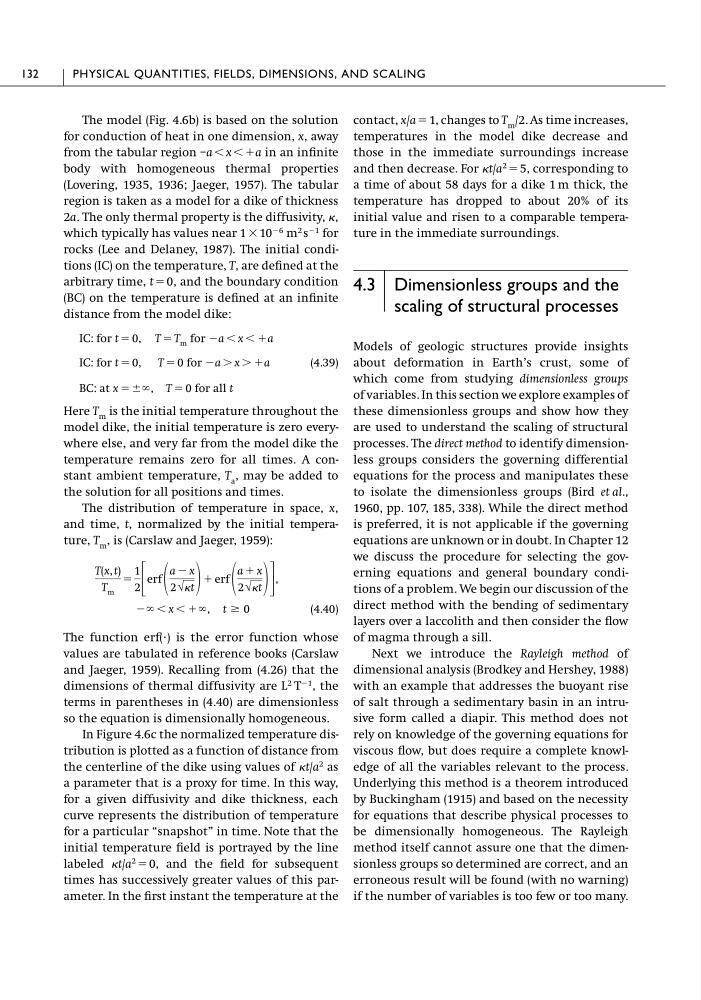
The model (Fig. 4.6b) is based on the solution
for conduction of heat in one dimension, x, away
from the tabular region –a Ͻ x Ͻϩa in an infinite
body with homogeneous thermal properties
(Lovering, 1935, 1936; Jaeger, 1957). The tabular
region is taken as a model for a dike of thickness
2a. The only thermal property is the diffusivity, ,
which typically has values near 1 ϫ 10
Ϫ6 m
2 s
Ϫ1 for
rocks (Lee and Delaney, 1987). The initial conditions (IC) on the temperature, T, are defined at the
arbitrary time, t ϭ 0, and the boundary condition
(BC) on the temperature is defined at an infinite
distance from the model dike:
(4.39)
Here T m is the initial temperature throughout the
model dike, the initial temperature is zero everywhere else, and very far from the model dike the
temperature remains zero for all times. A constant ambient temperature, T a , may be added to
the solution for all positions and times.
The distribution of temperature in space, x,
and time, t, normalized by the initial temperature, T m , is (Carslaw and Jaeger, 1959):
(4.40)
The function erf(и) is the error function whose
values are tabulated in reference books (Carslaw
and Jaeger, 1959). Recalling from (4.26) that the
dimensions of thermal diffusivity are L
2 T
Ϫ1 , the
terms in parentheses in (4.40) are dimensionless
so the equation is dimensionally homogeneous.
In Figure 4.6c the normalized temperature distribution is plotted as a function of distance from
the centerline of the dike using values of t/a
2 as
a parameter that is a proxy for time. In this way,
for a given diffusivity and dike thickness, each
curve represents the distribution of temperature
for a particular “snapshot” in time. Note that the
initial temperature field is portrayed by the line
labeled t/a
2 ϭ 0, and the field for subsequent
times has successively greater values of this parameter. In the first instant the temperature at the
Ϫϱ Ͻ x Ͻ ϩϱ, t Ն 0
T(x, t)
T m
ϭ
1
2 ΄ erf
a Ϫ x
2 √t ϩ erf
a ϩ x
2 √t ΅ ,
BC: at x ϭ Ϯϱ, T ϭ 0 for all t
IC: for t ϭ 0, T ϭ 0 for Ϫa Ͼ x Ͼ ϩa
IC: for t ϭ 0, T ϭ T m for Ϫa Ͻ x Ͻ ϩa
contact, x/a ϭ 1, changes to T m /2. As time increases,
temperatures in the model dike decrease and
those in the immediate surroundings increase
and then decrease. For t/a
2 ϭ 5, corresponding to
a time of about 58 days for a dike 1 m thick, the
temperature has dropped to about 20% of its
initial value and risen to a comparable temperature in the immediate surroundings.
4.3 Dimensionless groups and the
scaling of structural processes
Models of geologic structures provide insights
about deformation in Earth’s crust, some of
which come from studying dimensionless groups
of variables. In this section we explore examples of
these dimensionless groups and show how they
are used to understand the scaling of structural
processes. The direct method to identify dimensionless groups considers the governing differential
equations for the process and manipulates these
to isolate the dimensionless groups (Bird et al.,
1960, pp. 107, 185, 338). While the direct method
is preferred, it is not applicable if the governing
equations are unknown or in doubt. In Chapter 12
we discuss the procedure for selecting the governing equations and general boundary conditions of a problem. We begin our discussion of the
direct method with the bending of sedimentary
layers over a laccolith and then consider the flow
of magma through a sill.
Next we introduce the Rayleigh method of
dimensional analysis (Brodkey and Hershey, 1988)
with an example that addresses the buoyant rise
of salt through a sedimentary basin in an intrusive form called a diapir. This method does not
rely on knowledge of the governing equations for
viscous flow, but does require a complete knowledge of all the variables relevant to the process.
Underlying this method is a theorem introduced
by Buckingham (1915) and based on the necessity
for equations that describe physical processes to
be dimensionally homogeneous. The Rayleigh
method itself cannot assure one that the dimensionless groups so determined are correct, and an
erroneous result will be found (with no warning)
if the number of variables is too few or too many.
132
PHYSICAL QUANTITIES, FIELDS, DIMENSIONS, AND SCALING
for conduction of heat in one dimension, x, away
from the tabular region –a Ͻ x Ͻϩa in an infinite
body with homogeneous thermal properties
(Lovering, 1935, 1936; Jaeger, 1957). The tabular
region is taken as a model for a dike of thickness
2a. The only thermal property is the diffusivity, ,
which typically has values near 1 ϫ 10
Ϫ6 m
2 s
Ϫ1 for
rocks (Lee and Delaney, 1987). The initial conditions (IC) on the temperature, T, are defined at the
arbitrary time, t ϭ 0, and the boundary condition
(BC) on the temperature is defined at an infinite
distance from the model dike:
(4.39)
Here T m is the initial temperature throughout the
model dike, the initial temperature is zero everywhere else, and very far from the model dike the
temperature remains zero for all times. A constant ambient temperature, T a , may be added to
the solution for all positions and times.
The distribution of temperature in space, x,
and time, t, normalized by the initial temperature, T m , is (Carslaw and Jaeger, 1959):
(4.40)
The function erf(и) is the error function whose
values are tabulated in reference books (Carslaw
and Jaeger, 1959). Recalling from (4.26) that the
dimensions of thermal diffusivity are L
2 T
Ϫ1 , the
terms in parentheses in (4.40) are dimensionless
so the equation is dimensionally homogeneous.
In Figure 4.6c the normalized temperature distribution is plotted as a function of distance from
the centerline of the dike using values of t/a
2 as
a parameter that is a proxy for time. In this way,
for a given diffusivity and dike thickness, each
curve represents the distribution of temperature
for a particular “snapshot” in time. Note that the
initial temperature field is portrayed by the line
labeled t/a
2 ϭ 0, and the field for subsequent
times has successively greater values of this parameter. In the first instant the temperature at the
Ϫϱ Ͻ x Ͻ ϩϱ, t Ն 0
T(x, t)
T m
ϭ
1
2 ΄ erf
a Ϫ x
2 √t ϩ erf
a ϩ x
2 √t ΅ ,
BC: at x ϭ Ϯϱ, T ϭ 0 for all t
IC: for t ϭ 0, T ϭ 0 for Ϫa Ͼ x Ͼ ϩa
IC: for t ϭ 0, T ϭ T m for Ϫa Ͻ x Ͻ ϩa
contact, x/a ϭ 1, changes to T m /2. As time increases,
temperatures in the model dike decrease and
those in the immediate surroundings increase
and then decrease. For t/a
2 ϭ 5, corresponding to
a time of about 58 days for a dike 1 m thick, the
temperature has dropped to about 20% of its
initial value and risen to a comparable temperature in the immediate surroundings.
4.3 Dimensionless groups and the
scaling of structural processes
Models of geologic structures provide insights
about deformation in Earth’s crust, some of
which come from studying dimensionless groups
of variables. In this section we explore examples of
these dimensionless groups and show how they
are used to understand the scaling of structural
processes. The direct method to identify dimensionless groups considers the governing differential
equations for the process and manipulates these
to isolate the dimensionless groups (Bird et al.,
1960, pp. 107, 185, 338). While the direct method
is preferred, it is not applicable if the governing
equations are unknown or in doubt. In Chapter 12
we discuss the procedure for selecting the governing equations and general boundary conditions of a problem. We begin our discussion of the
direct method with the bending of sedimentary
layers over a laccolith and then consider the flow
of magma through a sill.
Next we introduce the Rayleigh method of
dimensional analysis (Brodkey and Hershey, 1988)
with an example that addresses the buoyant rise
of salt through a sedimentary basin in an intrusive form called a diapir. This method does not
rely on knowledge of the governing equations for
viscous flow, but does require a complete knowledge of all the variables relevant to the process.
Underlying this method is a theorem introduced
by Buckingham (1915) and based on the necessity
for equations that describe physical processes to
be dimensionally homogeneous. The Rayleigh
method itself cannot assure one that the dimensionless groups so determined are correct, and an
erroneous result will be found (with no warning)
if the number of variables is too few or too many.
132
PHYSICAL QUANTITIES, FIELDS, DIMENSIONS, AND SCALING