

just derived is useful, it is possible to represent the
“generic” model fault on a single curve by moving
the term 2(1 Ϫ )⌬/G to the left-hand side of (4.37):
(4.38)
Plotting the left-hand side as a function of the
right we generate the “generic” curve for dimensionless relative displacement versus dimensionless position (Fig. 4.5d). In this form one would
refer to the relative displacement as having been
normalized by the maximum relative displacement, 2(1 Ϫ )⌬/G, the value of the displacement
at the middle of the fault trace. The ends of the
fault are given by x/a ϭϩ1 and x/a ϭϪ1.
In Figure 4.5d the curve for relative displacement is symmetric and goes to zero at the ends of
the fault. At the middle of the fault, the offset of
geologic markers would be greatest and, on this
dimensionless graph, would have a magnitude of
ϩ1. All possible distributions of relative displacement for faults that approximate the behavior of
this theoretical model would scatter about a
single curve on this plot. The scatter would reflect
errors in measurement and mechanical differences between the model and natural fault. All of
the data sets for a set of faults could be plotted on
this graph and thereby could be compared to each
other and to the model.
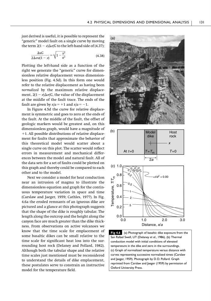
Next we consider a model for heat conduction
near an intrusion of magma to illustrate the
dimensionless equation and graph for the continuous temperature variation in space and time
(Carslaw and Jaeger, 1959; Cathles, 1977). In Fig.
4.6a the eroded remnants of an igneous dike are
pictured and a glance at this photograph suggests
that the shape of the dike is roughly tabular. The
length along the outcrop and the height along the
canyon face are much greater than the dike thickness. From observations on active volcanoes we
know that the time scale for emplacement of
some basaltic dikes can be small relative to the
time scale for significant heat loss into the surrounding host rock (Delaney and Pollard, 1982).
Although both the tabular shape and the relative
time scales just mentioned must be reconsidered
to understand the details of dike emplacement,
these postulates serve to constrain an instructive
model for the temperature field.
⌬uG
2⌬a(1 Ϫ )
ϭ
√
1 Ϫ
x 2
a 2
4.2 PHYSICAL DIMENSIONS AND DIMENSIONAL ANALYSIS
131
Fig 4.6 (a) Photograph of basaltic dike exposure from the
San Rafael Swell, UT (Delaney et al., 1986). (b) Thermal
conduction model with initial conditions of elevated
temperature in the dike and zero in the surroundings.
(c) Graph of normalized temperature versus distance with
curves representing successive normalized times (Carslaw
and Jaeger, 1959). Photograph by D. D. Pollard. Graph
reprinted from Carslaw and Jaeger (1959) by permission of
Oxford University Press.
1.0
0.8
0.6
0.4
0.2
0.0
2.0
1.0
3.0
Distance, x/a
Temperature,
T/T
m
0.0
1
2
5
0 .5
0 . 2
0
.0
1
(b)
x
2a
Model
dike
Host
rock
T =0
At t =0
(c)
0 . 1
0 . 0 5
0
.
0
2
kt/a 2 = 0.00
(a)
T =T m
Dike
“generic” model fault on a single curve by moving
the term 2(1 Ϫ )⌬/G to the left-hand side of (4.37):
(4.38)
Plotting the left-hand side as a function of the
right we generate the “generic” curve for dimensionless relative displacement versus dimensionless position (Fig. 4.5d). In this form one would
refer to the relative displacement as having been
normalized by the maximum relative displacement, 2(1 Ϫ )⌬/G, the value of the displacement
at the middle of the fault trace. The ends of the
fault are given by x/a ϭϩ1 and x/a ϭϪ1.
In Figure 4.5d the curve for relative displacement is symmetric and goes to zero at the ends of
the fault. At the middle of the fault, the offset of
geologic markers would be greatest and, on this
dimensionless graph, would have a magnitude of
ϩ1. All possible distributions of relative displacement for faults that approximate the behavior of
this theoretical model would scatter about a
single curve on this plot. The scatter would reflect
errors in measurement and mechanical differences between the model and natural fault. All of
the data sets for a set of faults could be plotted on
this graph and thereby could be compared to each
other and to the model.
Next we consider a model for heat conduction
near an intrusion of magma to illustrate the
dimensionless equation and graph for the continuous temperature variation in space and time
(Carslaw and Jaeger, 1959; Cathles, 1977). In Fig.
4.6a the eroded remnants of an igneous dike are
pictured and a glance at this photograph suggests
that the shape of the dike is roughly tabular. The
length along the outcrop and the height along the
canyon face are much greater than the dike thickness. From observations on active volcanoes we
know that the time scale for emplacement of
some basaltic dikes can be small relative to the
time scale for significant heat loss into the surrounding host rock (Delaney and Pollard, 1982).
Although both the tabular shape and the relative
time scales just mentioned must be reconsidered
to understand the details of dike emplacement,
these postulates serve to constrain an instructive
model for the temperature field.
⌬uG
2⌬a(1 Ϫ )
ϭ
√
1 Ϫ
x 2
a 2
4.2 PHYSICAL DIMENSIONS AND DIMENSIONAL ANALYSIS
131
Fig 4.6 (a) Photograph of basaltic dike exposure from the
San Rafael Swell, UT (Delaney et al., 1986). (b) Thermal
conduction model with initial conditions of elevated
temperature in the dike and zero in the surroundings.
(c) Graph of normalized temperature versus distance with
curves representing successive normalized times (Carslaw
and Jaeger, 1959). Photograph by D. D. Pollard. Graph
reprinted from Carslaw and Jaeger (1959) by permission of
Oxford University Press.
1.0
0.8
0.6
0.4
0.2
0.0
2.0
1.0
3.0
Distance, x/a
Temperature,
T/T
m
0.0
1
2
5
0 .5
0 . 2
0
.0
1
(b)
x
2a
Model
dike
Host
rock
T =0
At t =0
(c)
0 . 1
0 . 0 5
0
.
0
2
kt/a 2 = 0.00
(a)
T =T m
Dike