

fault during slip. Poisson’s ratio, , and the shear
modulus, G, are two properties of the elastic material surrounding the model fault. The combination G/(1 Ϫ ) can be thought of as the stiffness of
this material. Inspection of (4.29) shows that the
equation is dimensionally homogeneous. The
actual distribution of slip on faults and models to
explain these are part of a growing literature
(Cowie and Scholz, 1992; Dawers et al., 1993;
Bürgmann et al., 1994; Cowie and Shipton, 1998).
Because the origin of the coordinate system for
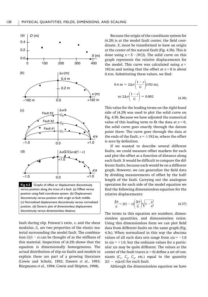
(4.29) is at the model fault center, the field coordinate, X, must be transformed to have an origin
at the center of the natural fault (Fig. 4.5b). This is
done using x ϭ X Ϫ (W/2). The solid curve on this
graph represents the relative displacements for
the model. This curve was calculated using a ϭ
192 m and noting that the offset at x ϭ 0 is about
0.4 m. Substituting these values, we find:
(4.36)
This value for the leading terms on the right-hand
side of (4.29) was used to plot the solid curve on
Fig. 4.5b. Because we have adjusted the numerical
value of this leading term to fit the data at x ϭ 0,
the solid curve goes exactly through the datum
point there. The curve goes through the data at
the ends of the fault, x ϭϮ192 m, where the offset
is zero by definition.
If we wanted to describe several different
faults, we could measure offset markers for each
and plot the offset as a function of distance along
each fault. It would be difficult to compare the different faults, because each would be on a different
graph. However, we can generalize the field data
by dividing measurements of offset by the halflength of the fault. Carrying out the analogous
operation for each side of the model equation we
find the following dimensionless equation for the
relative displacements:
(4.37)
The terms in this equation are numbers, dimensionless quantities, and dimensionless ratios.
Using this dimensionless form we can plot field
data from different faults on the same graph (Fig.
4.5c). When normalized in this way the abscissa
values of all such data sets range from x/a ϭϪ1.0
to x/a ϭϩ1.0, but the ordinate values for a particular x/a may be quite different. The values at the
center of the fault traces (x ϭ 0) define a set of constants (C 1 , C 2 , C 3 , etc.) equal to the quantity
2(1 Ϫ )⌬/G for each fault.
Although the dimensionless equation we have
⌬u
a
ϭ 2(1 Ϫ )
⌬
G √
1 Ϫ
x 2
a 2
so 2⌬
1 Ϫ
G Ϸ 0.002
0.4 m Ϸ 2⌬
1 Ϫ
G
(192 m),
130
PHYSICAL QUANTITIES, FIELDS, DIMENSIONS, AND SCALING
Fig 4.5 Graphs of offset or displacement discontinuity
versus position along the trace of a fault. (a) Offset versus
position using field coordinate system. (b) Displacement
discontinuity versus position with origin at fault middle.
(c) Normalized displacement discontinuity versus normalized
position. (d) Generic plot of dimensionless displacement
discontinuity versus dimensionless distance.
(a)
400
0
X (m)
O (m)
(b)
+192 m
–192 m
0.0
0.4 m
x (m)
⌬u (m)
0.2 m
0.4
0.2
0.0
300
200
100
+1.0
–1.0
0.0
+1.0
(d)
+1.0
–1.0
0.0
x/a
(c)
C 3
C 2
C 1
Fault #2
Fault #3
Fault #1
⌬u/a
x/a
⌬uG/2⌬a(1 – n)
modulus, G, are two properties of the elastic material surrounding the model fault. The combination G/(1 Ϫ ) can be thought of as the stiffness of
this material. Inspection of (4.29) shows that the
equation is dimensionally homogeneous. The
actual distribution of slip on faults and models to
explain these are part of a growing literature
(Cowie and Scholz, 1992; Dawers et al., 1993;
Bürgmann et al., 1994; Cowie and Shipton, 1998).
Because the origin of the coordinate system for
(4.29) is at the model fault center, the field coordinate, X, must be transformed to have an origin
at the center of the natural fault (Fig. 4.5b). This is
done using x ϭ X Ϫ (W/2). The solid curve on this
graph represents the relative displacements for
the model. This curve was calculated using a ϭ
192 m and noting that the offset at x ϭ 0 is about
0.4 m. Substituting these values, we find:
(4.36)
This value for the leading terms on the right-hand
side of (4.29) was used to plot the solid curve on
Fig. 4.5b. Because we have adjusted the numerical
value of this leading term to fit the data at x ϭ 0,
the solid curve goes exactly through the datum
point there. The curve goes through the data at
the ends of the fault, x ϭϮ192 m, where the offset
is zero by definition.
If we wanted to describe several different
faults, we could measure offset markers for each
and plot the offset as a function of distance along
each fault. It would be difficult to compare the different faults, because each would be on a different
graph. However, we can generalize the field data
by dividing measurements of offset by the halflength of the fault. Carrying out the analogous
operation for each side of the model equation we
find the following dimensionless equation for the
relative displacements:
(4.37)
The terms in this equation are numbers, dimensionless quantities, and dimensionless ratios.
Using this dimensionless form we can plot field
data from different faults on the same graph (Fig.
4.5c). When normalized in this way the abscissa
values of all such data sets range from x/a ϭϪ1.0
to x/a ϭϩ1.0, but the ordinate values for a particular x/a may be quite different. The values at the
center of the fault traces (x ϭ 0) define a set of constants (C 1 , C 2 , C 3 , etc.) equal to the quantity
2(1 Ϫ )⌬/G for each fault.
Although the dimensionless equation we have
⌬u
a
ϭ 2(1 Ϫ )
⌬
G √
1 Ϫ
x 2
a 2
so 2⌬
1 Ϫ
G Ϸ 0.002
0.4 m Ϸ 2⌬
1 Ϫ
G
(192 m),
130
PHYSICAL QUANTITIES, FIELDS, DIMENSIONS, AND SCALING
Fig 4.5 Graphs of offset or displacement discontinuity
versus position along the trace of a fault. (a) Offset versus
position using field coordinate system. (b) Displacement
discontinuity versus position with origin at fault middle.
(c) Normalized displacement discontinuity versus normalized
position. (d) Generic plot of dimensionless displacement
discontinuity versus dimensionless distance.
(a)
400
0
X (m)
O (m)
(b)
+192 m
–192 m
0.0
0.4 m
x (m)
⌬u (m)
0.2 m
0.4
0.2
0.0
300
200
100
+1.0
–1.0
0.0
+1.0
(d)
+1.0
–1.0
0.0
x/a
(c)
C 3
C 2
C 1
Fault #2
Fault #3
Fault #1
⌬u/a
x/a
⌬uG/2⌬a(1 – n)