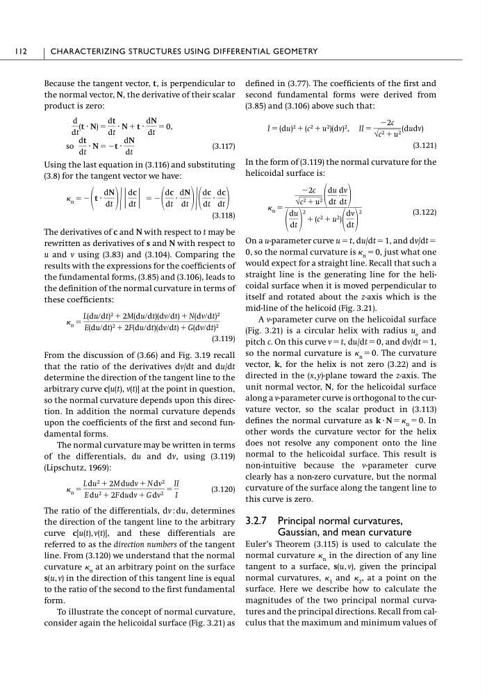
Because the tangent vector, t, is perpendicular to
the normal vector, N, the derivative of their scalar
product is zero:
(3.117)
Using the last equation in (3.116) and substituting
(3.8) for the tangent vector we have:
(3.118)
The derivatives of c and N with respect to t may be
rewritten as derivatives of s and N with respect to
u and v using (3.83) and (3.104). Comparing the
results with the expressions for the coefficients of
the fundamental forms, (3.85) and (3.106), leads to
the definition of the normal curvature in terms of
these coefficients:
(3.119)
From the discussion of (3.66) and Fig. 3.19 recall
that the ratio of the derivatives dv/dt and du/dt
determine the direction of the tangent line to the
arbitrary curve c[u(t), v(t)] at the point in question,
so the normal curvature depends upon this direction. In addition the normal curvature depends
upon the coefficients of the first and second fundamental forms.
The normal curvature may be written in terms
of the differentials, du and dv, using (3.119)
(Lipschutz, 1969):
(3.120)
The ratio of the differentials, dv : du, determines
the direction of the tangent line to the arbitrary
curve c[u(t), v(t)], and these differentials are
referred to as the direction numbers of the tangent
line. From (3.120) we understand that the normal
curvature ␬ n at an arbitrary point on the surface
s(u, v) in the direction of this tangent line is equal
to the ratio of the second to the first fundamental
form.
To illustrate the concept of normal curvature,
consider again the helicoidal surface (Fig. 3.21) as
␬ n ϭ
L du 2 ϩ 2M dudv ϩ N dv 2
E du 2 ϩ 2F dudv ϩ G dv 2 ϭ
II
I
␬ n ϭ
L(duրdt) 2 ϩ 2M(duրdt)(dvրdt) ϩ N(dvրdt) 2
E(duրdt) 2 ϩ 2F(duրdt)(dvրdt) ϩ G(dvրdt) 2
ϭ Ϫ ΂
dc
dt
·
dN
dt ΃/΂
dc
dt
·
dc
dt ΃
␬ n ϭ Ϫ ΂ t ·
dN
dt ΃/ |
dc
dt |
so 
dt
dt
· N ϭ Ϫt ·
dN
dt
d
dt
(t · N) ϭ
dt
dt
· N ϩ t ·
dN
dt
ϭ 0,
defined in (3.77). The coefficients of the first and
second fundamental forms were derived from
(3.85) and (3.106) above such that:
(3.121)
In the form of (3.119) the normal curvature for the
helicoidal surface is:
(3.122)
On a u-parameter curve u ϭ t, du/dt ϭ 1, and dv/dt ϭ
0, so the normal curvature is ␬ n ϭ 0, just what one
would expect for a straight line. Recall that such a
straight line is the generating line for the helicoidal surface when it is moved perpendicular to
itself and rotated about the z-axis which is the
mid-line of the helicoid (Fig. 3.21).
A v-parameter curve on the helicoidal surface
(Fig. 3.21) is a circular helix with radius u o and
pitch c. On this curve v ϭ t, du/dt ϭ 0, and dv/dt ϭ 1,
so the normal curvature is ␬ n ϭ 0. The curvature
vector, k, for the helix is not zero (3.22) and is
directed in the (x, y)-plane toward the z-axis. The
unit normal vector, N, for the helicoidal surface
along a v-parameter curve is orthogonal to the curvature vector, so the scalar product in (3.113)
defines the normal curvature as k иN ϭ ␬ n ϭ 0. In
other words the curvature vector for the helix
does not resolve any component onto the line
normal to the helicoidal surface. This result is
non-intuitive because the v-parameter curve
clearly has a non-zero curvature, but the normal
curvature of the surface along the tangent line to
this curve is zero.
3.2.7 Principal normal curvatures,
Gaussian, and mean curvature
Euler’s Theorem (3.115) is used to calculate the
normal curvature ␬ n in the direction of any line
tangent to a surface, s(u, v), given the principal
normal curvatures, ␬ 1 and ␬ 2 , at a point on the
surface. Here we describe how to calculate the
magnitudes of the two principal normal curvatures and the principal directions. Recall from calculus that the maximum and minimum values of
␬ n ϭ
Ϫ2c
√c 2 ϩ u 2 ΂
du
dt
dv
dt ΃
΂
du
dt ΃
2
ϩ (c 2 ϩ u 2 )
΂
dv
dt ΃
2
I ϭ (du) 2 ϩ (c 2 ϩ u 2 )(dv) 2 ,  II ϭ
Ϫ2c
√c 2 ϩ u 2 (dudv)
112
CHARACTERIZING STRUCTURES USING DIFFERENTIAL GEOMETRY