

The variation of normal curvature with direction is of the same form for all surfaces with
continuous second partial derivatives such that
(Lipschutz, 1969):
(3.115)
This relationship is known as Euler’s Theorem and
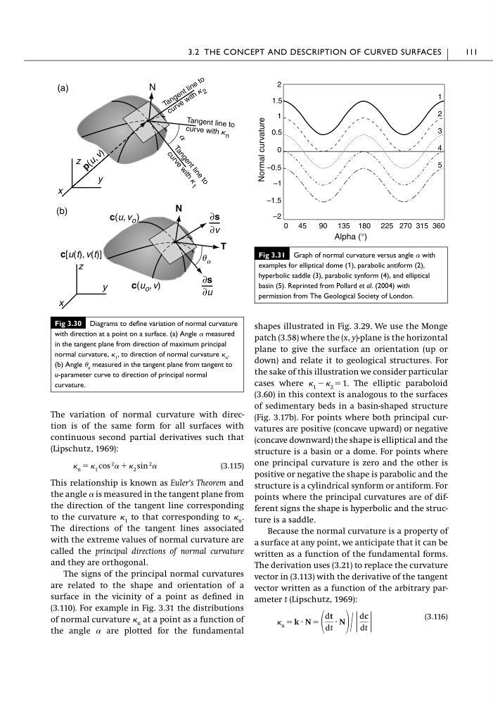
the angle ␣ is measured in the tangent plane from
the direction of the tangent line corresponding
to the curvature 1 to that corresponding to n .
The directions of the tangent lines associated
with the extreme values of normal curvature are
called the principal directions of normal curvature
and they are orthogonal.
The signs of the principal normal curvatures
are related to the shape and orientation of a
surface in the vicinity of a point as defined in
(3.110). For example in Fig. 3.31 the distributions
of normal curvature n at a point as a function of
the angle ␣ are plotted for the fundamental
n ϭ 1 cos
2 ␣ ϩ 2 sin
2 ␣
shapes illustrated in Fig. 3.29. We use the Monge
patch (3.58) where the (x, y)-plane is the horizontal
plane to give the surface an orientation (up or
down) and relate it to geological structures. For
the sake of this illustration we consider particular
cases where 1 Ϫ 2 ϭ 1. The elliptic paraboloid
(3.60) in this context is analogous to the surfaces
of sedimentary beds in a basin-shaped structure
(Fig. 3.17b). For points where both principal curvatures are positive (concave upward) or negative
(concave downward) the shape is elliptical and the
structure is a basin or a dome. For points where
one principal curvature is zero and the other is
positive or negative the shape is parabolic and the
structure is a cylindrical synform or antiform. For
points where the principal curvatures are of different signs the shape is hyperbolic and the structure is a saddle.
Because the normal curvature is a property of
a surface at any point, we anticipate that it can be
written as a function of the fundamental forms.
The derivation uses (3.21) to replace the curvature
vector in (3.113) with the derivative of the tangent
vector written as a function of the arbitrary parameter t (Lipschutz, 1969):
(3.116)
n ϭ k · N ϭ
dt
dt
· N ր |
dc
dt |
3.2 THE CONCEPT AND DESCRIPTION OF CURVED SURFACES
111
Fig 3.30 Diagrams to define variation of normal curvature
with direction at a point on a surface. (a) Angle ␣ measured
in the tangent plane from direction of maximum principal
normal curvature, 1 , to direction of normal curvature n .
(b) Angle o measured in the tangent plane from tangent to
u-parameter curve to direction of principal normal
curvature.
y
z
x
(a)
N
a
T a n g e n t l i n e
t o
c u r v e
w i t h
K 1
T a n g e n t li n e t o
c u r v e w it h K 2
Tan gen t line to
cur ve with K n
y
z
x
(b)
∂u
∂s
∂v
∂s
N
T
p ( u , v )
c(u o , v)
c[u(t), v(t)]
c(u, v o )
U o
Fig 3.31 Graph of normal curvature versus angle ␣ with
examples for elliptical dome (1), parabolic antiform (2),
hyperbolic saddle (3), parabolic synform (4), and elliptical
basin (5). Reprinted from Pollard et al. (2004) with
permission from The Geological Society of London.
0
1
1
2
3
4
5
2
Normal curvature
Alpha (°)
1.5
0.5
–0.5
–1
–1.5
–2
0 45
90 135 180 225 270 315 360
continuous second partial derivatives such that
(Lipschutz, 1969):
(3.115)
This relationship is known as Euler’s Theorem and
the angle ␣ is measured in the tangent plane from
the direction of the tangent line corresponding
to the curvature 1 to that corresponding to n .
The directions of the tangent lines associated
with the extreme values of normal curvature are
called the principal directions of normal curvature
and they are orthogonal.
The signs of the principal normal curvatures
are related to the shape and orientation of a
surface in the vicinity of a point as defined in
(3.110). For example in Fig. 3.31 the distributions
of normal curvature n at a point as a function of
the angle ␣ are plotted for the fundamental
n ϭ 1 cos
2 ␣ ϩ 2 sin
2 ␣
shapes illustrated in Fig. 3.29. We use the Monge
patch (3.58) where the (x, y)-plane is the horizontal
plane to give the surface an orientation (up or
down) and relate it to geological structures. For
the sake of this illustration we consider particular
cases where 1 Ϫ 2 ϭ 1. The elliptic paraboloid
(3.60) in this context is analogous to the surfaces
of sedimentary beds in a basin-shaped structure
(Fig. 3.17b). For points where both principal curvatures are positive (concave upward) or negative
(concave downward) the shape is elliptical and the
structure is a basin or a dome. For points where
one principal curvature is zero and the other is
positive or negative the shape is parabolic and the
structure is a cylindrical synform or antiform. For
points where the principal curvatures are of different signs the shape is hyperbolic and the structure is a saddle.
Because the normal curvature is a property of
a surface at any point, we anticipate that it can be
written as a function of the fundamental forms.
The derivation uses (3.21) to replace the curvature
vector in (3.113) with the derivative of the tangent
vector written as a function of the arbitrary parameter t (Lipschutz, 1969):
(3.116)
n ϭ k · N ϭ
dt
dt
· N ր |
dc
dt |
3.2 THE CONCEPT AND DESCRIPTION OF CURVED SURFACES
111
Fig 3.30 Diagrams to define variation of normal curvature
with direction at a point on a surface. (a) Angle ␣ measured
in the tangent plane from direction of maximum principal
normal curvature, 1 , to direction of normal curvature n .
(b) Angle o measured in the tangent plane from tangent to
u-parameter curve to direction of principal normal
curvature.
y
z
x
(a)
N
a
T a n g e n t l i n e
t o
c u r v e
w i t h
K 1
T a n g e n t li n e t o
c u r v e w it h K 2
Tan gen t line to
cur ve with K n
y
z
x
(b)
∂u
∂s
∂v
∂s
N
T
p ( u , v )
c(u o , v)
c[u(t), v(t)]
c(u, v o )
U o
Fig 3.31 Graph of normal curvature versus angle ␣ with
examples for elliptical dome (1), parabolic antiform (2),
hyperbolic saddle (3), parabolic synform (4), and elliptical
basin (5). Reprinted from Pollard et al. (2004) with
permission from The Geological Society of London.
0
1
1
2
3
4
5
2
Normal curvature
Alpha (°)
1.5
0.5
–0.5
–1
–1.5
–2
0 45
90 135 180 225 270 315 360