

Similar expansions yield the other coefficients of
the second fundamental:
(3.109)
These coefficients are the scalar product of the
unit normal vector and the respective second
partial derivatives of the surface, s(u, v).
One can use the coefficients of the second fundamental form to characterize the shape of a
surface in the vicinity of a particular point as
follows (Lipschutz, 1969):
(3.110)
For the parabolic point not all of the coefficients
are zero but the combination LNϪM
2 is zero. The
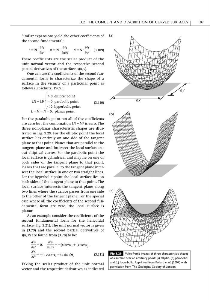
three non-planar characteristic shapes are illustrated in Fig. 3.29. For the elliptic point the local
surface lies entirely on one side of the tangent
plane to that point. Planes that are parallel to the
tangent plane and intersect the local surface cut
out elliptical curves. For the parabolic point the
local surface is cylindrical and may lie on one or
both sides of the tangent plane to that point.
Planes that are parallel to the tangent plane intersect the local surface in one or two straight lines.
For the hyperbolic point the local surface lies on
both sides of the tangent plane to that point. The
local surface intersects the tangent plane along
two lines where the surface passes from one side
to the other of the tangent plane. For the special
case where all the coefficients of the second fundamental form are zero, the local surface is
planar.
As an example consider the coefficients of the
second fundamental form for the helicoidal
surface (Fig. 3.21). The unit normal vector is given
in (3.79) and the second partial derivatives of
s(u, v) are found from (3.78) to be:
(3.111)
Taking the scalar product of the unit normal
vector and the respective derivatives as indicated
Ѩ
2 s
Ѩv
2
ϭ Ϫ(u cos v)e x Ϫ (u sin v)e y
Ѩ
2 s
Ѩu
2
ϭ 0,
Ѩ
2 s
ѨuѨv
ϭ Ϫ( sin v)e x ϩ ( cos v)e y ,
L ϭ M ϭ N ϭ 0, planar point
LN Ϫ M 2
Ά
Ͼ 0, elliptic point
ϭ 0, parabolic point
Ͻ 0, hyperbolic point
L ϭ N ·
Ѩ
2 s
Ѩu
2
, M ϭ N ·
Ѩ
2
s
ѨuѨv
, N ϭ N ·
Ѩ
2 s
Ѩv
2
3.2 THE CONCEPT AND DESCRIPTION OF CURVED SURFACES
109
Fig 3.29 Wire-frame images of three characteristic shapes
of a surface near an arbitrary point: (a) elliptic, (b) parabolic,
and (c) hyperbolic. Reprinted from Pollard et al. (2004) with
permission from The Geological Society of London.
the second fundamental:
(3.109)
These coefficients are the scalar product of the
unit normal vector and the respective second
partial derivatives of the surface, s(u, v).
One can use the coefficients of the second fundamental form to characterize the shape of a
surface in the vicinity of a particular point as
follows (Lipschutz, 1969):
(3.110)
For the parabolic point not all of the coefficients
are zero but the combination LNϪM
2 is zero. The
three non-planar characteristic shapes are illustrated in Fig. 3.29. For the elliptic point the local
surface lies entirely on one side of the tangent
plane to that point. Planes that are parallel to the
tangent plane and intersect the local surface cut
out elliptical curves. For the parabolic point the
local surface is cylindrical and may lie on one or
both sides of the tangent plane to that point.
Planes that are parallel to the tangent plane intersect the local surface in one or two straight lines.
For the hyperbolic point the local surface lies on
both sides of the tangent plane to that point. The
local surface intersects the tangent plane along
two lines where the surface passes from one side
to the other of the tangent plane. For the special
case where all the coefficients of the second fundamental form are zero, the local surface is
planar.
As an example consider the coefficients of the
second fundamental form for the helicoidal
surface (Fig. 3.21). The unit normal vector is given
in (3.79) and the second partial derivatives of
s(u, v) are found from (3.78) to be:
(3.111)
Taking the scalar product of the unit normal
vector and the respective derivatives as indicated
Ѩ
2 s
Ѩv
2
ϭ Ϫ(u cos v)e x Ϫ (u sin v)e y
Ѩ
2 s
Ѩu
2
ϭ 0,
Ѩ
2 s
ѨuѨv
ϭ Ϫ( sin v)e x ϩ ( cos v)e y ,
L ϭ M ϭ N ϭ 0, planar point
LN Ϫ M 2
Ά
Ͼ 0, elliptic point
ϭ 0, parabolic point
Ͻ 0, hyperbolic point
L ϭ N ·
Ѩ
2 s
Ѩu
2
, M ϭ N ·
Ѩ
2
s
ѨuѨv
, N ϭ N ·
Ѩ
2 s
Ѩv
2
3.2 THE CONCEPT AND DESCRIPTION OF CURVED SURFACES
109
Fig 3.29 Wire-frame images of three characteristic shapes
of a surface near an arbitrary point: (a) elliptic, (b) parabolic,
and (c) hyperbolic. Reprinted from Pollard et al. (2004) with
permission from The Geological Society of London.