

Again we see that the curvature is not simply
related to the second derivative of the vector function c(t).
The circular helix is not a planar curve, so we
turn to the parametric representation of a parabolic curve that lies entirely in the (x, y)-plane (Fig.
3.10b):
(3.35)
Taking the first and second derivatives of the components, the scalar curvature is found using
(3.34):
(3.36)
For t ϭϪ0.5 we find ϭ 0.707 so ϭ 1.414 and a
circle of this radius is shown tangent to the
parabola at this point in Fig. 3.10b. For t ϭ 0 the
scalar curvature ϭ 2 and the radius of curvature
is ϭ 0.5. A circle with this radius of curvature is
shown tangent to the point at the base of the
parabola. Clearly there is a significant change in
curvature along a relatively short arc of the
parabola.
We further specialize the representation of
the curve such that c x (x) ϭ x and c y (x) ϭ y. In other
words the arbitrary parameter in (3.33) is the xcoordinate, and the derivatives of the two components of c may be rewritten:
(3.37)
Upon substitution into (3.34) the curvature takes
the form often introduced in calculus textbooks
(Varberg and Purcell, 1992, p. 623):
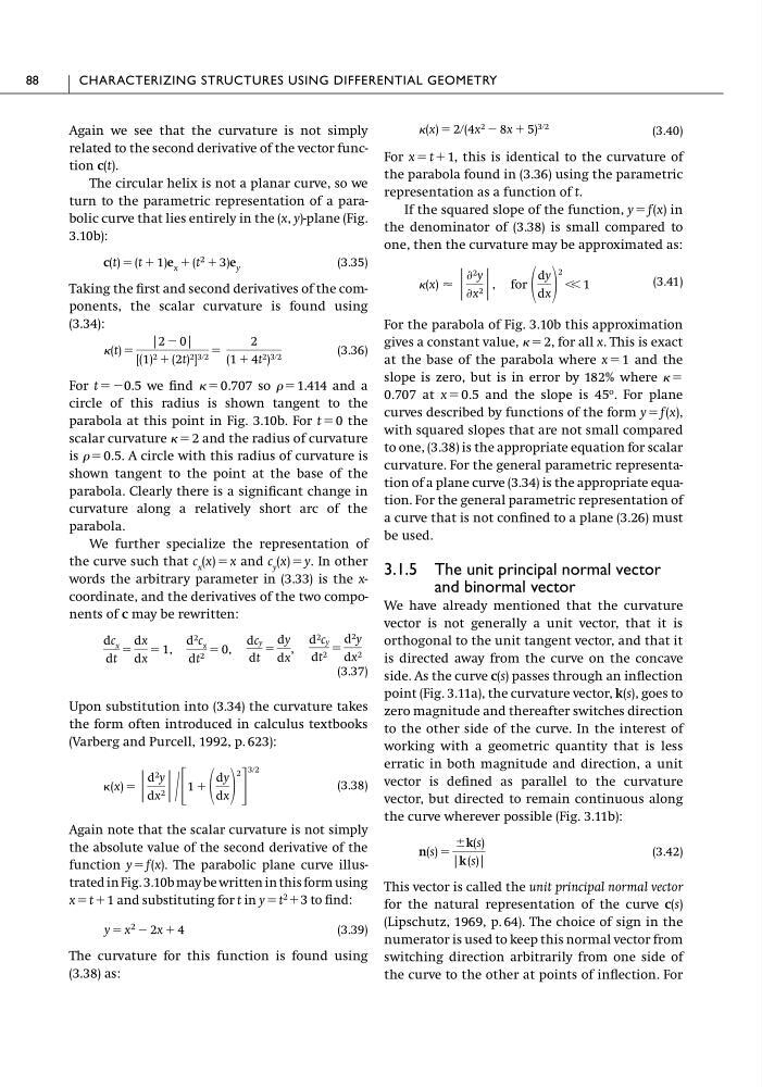
(3.38)
Again note that the scalar curvature is not simply
the absolute value of the second derivative of the
function y ϭ f(x). The parabolic plane curve illustrated in Fig. 3.10b may be written in this form using
x ϭ tϩ1 and substituting for t in y ϭ t
2 ϩ3 to find:
(3.39)
The curvature for this function is found using
(3.38) as:
y ϭ x 2 Ϫ 2x ϩ 4
(x) ϭ |
d 2 y
dx 2 | ր ΄
1 ϩ
dy
dx
2
΅
3ր2
dc x
dt
ϭ
dx
dx
ϭ 1,
d 2 c x
dt 2 ϭ 0,
dcy
dt
ϭ
dy
dx
,
d 2 cy
dt 2 ϭ
d 2 y
dx 2
(t) ϭ
|2 Ϫ 0|
[(1) 2 ϩ (2t) 2 ] 3ր2 ϭ
2
(1 ϩ 4t 2 ) 3ր2
c(t) ϭ (t ϩ 1)e x ϩ (t 2 ϩ 3)e y
(3.40)
For x ϭ tϩ1, this is identical to the curvature of
the parabola found in (3.36) using the parametric
representation as a function of t.
If the squared slope of the function, y ϭ f(x) in
the denominator of (3.38) is small compared to
one, then the curvature may be approximated as:
(3.41)
For the parabola of Fig. 3.10b this approximation
gives a constant value, ϭ 2, for all x. This is exact
at the base of the parabola where x ϭ 1 and the
slope is zero, but is in error by 182% where ϭ
0.707 at x ϭ 0.5 and the slope is 45
o
. For plane
curves described by functions of the form y ϭ f(x),
with squared slopes that are not small compared
to one, (3.38) is the appropriate equation for scalar
curvature. For the general parametric representation of a plane curve (3.34) is the appropriate equation. For the general parametric representation of
a curve that is not confined to a plane (3.26) must
be used.
3.1.5 The unit principal normal vector
and binormal vector
We have already mentioned that the curvature
vector is not generally a unit vector, that it is
orthogonal to the unit tangent vector, and that it
is directed away from the curve on the concave
side. As the curve c(s) passes through an inflection
point (Fig. 3.11a), the curvature vector, k(s), goes to
zero magnitude and thereafter switches direction
to the other side of the curve. In the interest of
working with a geometric quantity that is less
erratic in both magnitude and direction, a unit
vector is defined as parallel to the curvature
vector, but directed to remain continuous along
the curve wherever possible (Fig. 3.11b):
(3.42)
This vector is called the unit principal normal vector
for the natural representation of the curve c(s)
(Lipschutz, 1969, p. 64). The choice of sign in the
numerator is used to keep this normal vector from
switching direction arbitrarily from one side of
the curve to the other at points of inflection. For
n(s) ϭ
Ϯk(s)
|k (s)|
(x) Ϸ |
Ѩ 2 y
Ѩx 2 | , for
dy
dx
2
Ͻ Ͻ 1
(x) ϭ 2ր(4x 2 Ϫ 8x ϩ 5) 3ր2
88
CHARACTERIZING STRUCTURES USING DIFFERENTIAL GEOMETRY
related to the second derivative of the vector function c(t).
The circular helix is not a planar curve, so we
turn to the parametric representation of a parabolic curve that lies entirely in the (x, y)-plane (Fig.
3.10b):
(3.35)
Taking the first and second derivatives of the components, the scalar curvature is found using
(3.34):
(3.36)
For t ϭϪ0.5 we find ϭ 0.707 so ϭ 1.414 and a
circle of this radius is shown tangent to the
parabola at this point in Fig. 3.10b. For t ϭ 0 the
scalar curvature ϭ 2 and the radius of curvature
is ϭ 0.5. A circle with this radius of curvature is
shown tangent to the point at the base of the
parabola. Clearly there is a significant change in
curvature along a relatively short arc of the
parabola.
We further specialize the representation of
the curve such that c x (x) ϭ x and c y (x) ϭ y. In other
words the arbitrary parameter in (3.33) is the xcoordinate, and the derivatives of the two components of c may be rewritten:
(3.37)
Upon substitution into (3.34) the curvature takes
the form often introduced in calculus textbooks
(Varberg and Purcell, 1992, p. 623):
(3.38)
Again note that the scalar curvature is not simply
the absolute value of the second derivative of the
function y ϭ f(x). The parabolic plane curve illustrated in Fig. 3.10b may be written in this form using
x ϭ tϩ1 and substituting for t in y ϭ t
2 ϩ3 to find:
(3.39)
The curvature for this function is found using
(3.38) as:
y ϭ x 2 Ϫ 2x ϩ 4
(x) ϭ |
d 2 y
dx 2 | ր ΄
1 ϩ
dy
dx
2
΅
3ր2
dc x
dt
ϭ
dx
dx
ϭ 1,
d 2 c x
dt 2 ϭ 0,
dcy
dt
ϭ
dy
dx
,
d 2 cy
dt 2 ϭ
d 2 y
dx 2
(t) ϭ
|2 Ϫ 0|
[(1) 2 ϩ (2t) 2 ] 3ր2 ϭ
2
(1 ϩ 4t 2 ) 3ր2
c(t) ϭ (t ϩ 1)e x ϩ (t 2 ϩ 3)e y
(3.40)
For x ϭ tϩ1, this is identical to the curvature of
the parabola found in (3.36) using the parametric
representation as a function of t.
If the squared slope of the function, y ϭ f(x) in
the denominator of (3.38) is small compared to
one, then the curvature may be approximated as:
(3.41)
For the parabola of Fig. 3.10b this approximation
gives a constant value, ϭ 2, for all x. This is exact
at the base of the parabola where x ϭ 1 and the
slope is zero, but is in error by 182% where ϭ
0.707 at x ϭ 0.5 and the slope is 45
o
. For plane
curves described by functions of the form y ϭ f(x),
with squared slopes that are not small compared
to one, (3.38) is the appropriate equation for scalar
curvature. For the general parametric representation of a plane curve (3.34) is the appropriate equation. For the general parametric representation of
a curve that is not confined to a plane (3.26) must
be used.
3.1.5 The unit principal normal vector
and binormal vector
We have already mentioned that the curvature
vector is not generally a unit vector, that it is
orthogonal to the unit tangent vector, and that it
is directed away from the curve on the concave
side. As the curve c(s) passes through an inflection
point (Fig. 3.11a), the curvature vector, k(s), goes to
zero magnitude and thereafter switches direction
to the other side of the curve. In the interest of
working with a geometric quantity that is less
erratic in both magnitude and direction, a unit
vector is defined as parallel to the curvature
vector, but directed to remain continuous along
the curve wherever possible (Fig. 3.11b):
(3.42)
This vector is called the unit principal normal vector
for the natural representation of the curve c(s)
(Lipschutz, 1969, p. 64). The choice of sign in the
numerator is used to keep this normal vector from
switching direction arbitrarily from one side of
the curve to the other at points of inflection. For
n(s) ϭ
Ϯk(s)
|k (s)|
(x) Ϸ |
Ѩ 2 y
Ѩx 2 | , for
dy
dx
2
Ͻ Ͻ 1
(x) ϭ 2ր(4x 2 Ϫ 8x ϩ 5) 3ր2
88
CHARACTERIZING STRUCTURES USING DIFFERENTIAL GEOMETRY