

curve are identical at the point c(s). The circle C is
the one circle, of an infinite number of different
circles that pass through this point, that has the
closest contact with the curve, and therefore provides a geometric visualization of the radius of
curvature. One can say that it is the “best-fitting”
circle to the curve at that point.
For the natural representation of a curve, c(s),
recall that the curvature vector is the second
derivative of the position vector: k(s) ϭ d
2 c/ds
2 , so
the scalar curvature is defined as (s) ϭ |d
2 c/ds
2 |.
Given this definition, one might be tempted to
associate curvature with the second derivative of
a function, say y ϭ f(x), representing a plane curve.
In fact, this is commonly done in casual conversations where one says the first derivative, dy/dx, is
the slope of the curve, and the second derivative,
d
2 y/dx
2 , is the curvature. However, such statements involve special conditions and approximations that are spelled out in the following
paragraphs.
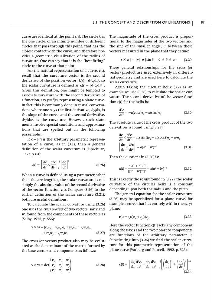
If c ϭ c(t) is the arbitrary parametric representation of a curve, as in (3.1), then a general
definition of the scalar curvature is (Lipschutz,
1969, p. 64):
(3.26)
When a curve is defined using a parameter other
then the arc length, s, the scalar curvature is not
simply the absolute value of the second derivative
of the vector function c(t). Compare (3.26) to the
earlier definition of the scalar curvature (3.21):
both are useful definitions.
To calculate the scalar curvature using (3.26)
one uses the cross product of two vectors, say v and
w, found from the components of these vectors as
(Selby, 1975, p. 556):
(3.27)
The cross (or vector) product also may be evaluated as the determinant of the matrix formed by
the base vectors and components as follows:
(3.28)
v ϫ w ϭ det
e x v x w x
e y v y w y
e z v z w z
ϩ (v x w y Ϫ v y w x )e z
v ϫ w ϭ (v y w z Ϫ v z w y )e x ϩ (v z w x Ϫ v x w z )e y
(t) ϭ |
dc
dt
ϫ
d 2 c
dt 2 | ր |
dc
dt |
3
The magnitude of the cross product is proportional to the magnitudes of the two vectors and
the sine of the smaller angle, , between these
vectors measured in the plane that they define:
(3.29)
These general relationships for the cross (or
vector) product are used extensively in differential geometry and are used here to calculate the
scalar curvature.
Again taking the circular helix (3.2) as an
example we use (3.26) to calculate the scalar curvature. The second derivative of the vector function c(t) for the helix is:
(3.30)
The absolute value of the cross product of the two
derivatives is found using (3.27):
(3.31)
Then the quotient in (3.26) is:
(3.32)
This is exactly the result found in (3.22): the scalar
curvature of the circular helix is a constant
depending upon both the radius and the pitch.
The general equation for the scalar curvature
(3.26) may be specialized for a plane curve, for
example a curve that lies entirely within the (x, y)plane:
(3.33)
Here the vector function c(t) lacks any component
along the z-axis and the two non-zero components
are functions of the arbitrary parameter, t.
Substituting into (3.26) we find the scalar curvature for this parametric representation of the
plane curve (Varberg and Purcell, 1992, p. 623):
(3.34)
(t) ϭ |
dc x
dt
d 2 cy
dt 2 Ϫ
dcy
dt
d 2 c x
dt 2 | ր ΄
dc x
dt
2
ϩ
dc y
dt
2
΅
3ր2
c(t) ϭ c x (t)e x ϩ c y (t)e y
(t) ϭ
a(a 2 ϩ b 2 ) 1ր2
[(a 2 ϩ b 2 ) 1ր2 ] 3 ϭ a(a 2 ϩ b 2 ) Ϫ1
|
dc
dt
ϫ
d 2 c
dt 2 | ϭ a(a 2 ϩ b 2 ) 1ր2
dc
dt
ϫ
d 2 c
dt 2 ϭ ab( sin t)e x Ϫ ab( cos t)e y ϩ a 2 e z
d 2 c
dt 2 ϭ Ϫa(cos t)e x Ϫ a(sin t)e y
|v ϫ w| ϭ |v||w|sin , 0 Յ Յ
3.1 THE CONCEPT AND DESCRIPTION OF LINEATIONS
87
the one circle, of an infinite number of different
circles that pass through this point, that has the
closest contact with the curve, and therefore provides a geometric visualization of the radius of
curvature. One can say that it is the “best-fitting”
circle to the curve at that point.
For the natural representation of a curve, c(s),
recall that the curvature vector is the second
derivative of the position vector: k(s) ϭ d
2 c/ds
2 , so
the scalar curvature is defined as (s) ϭ |d
2 c/ds
2 |.
Given this definition, one might be tempted to
associate curvature with the second derivative of
a function, say y ϭ f(x), representing a plane curve.
In fact, this is commonly done in casual conversations where one says the first derivative, dy/dx, is
the slope of the curve, and the second derivative,
d
2 y/dx
2 , is the curvature. However, such statements involve special conditions and approximations that are spelled out in the following
paragraphs.
If c ϭ c(t) is the arbitrary parametric representation of a curve, as in (3.1), then a general
definition of the scalar curvature is (Lipschutz,
1969, p. 64):
(3.26)
When a curve is defined using a parameter other
then the arc length, s, the scalar curvature is not
simply the absolute value of the second derivative
of the vector function c(t). Compare (3.26) to the
earlier definition of the scalar curvature (3.21):
both are useful definitions.
To calculate the scalar curvature using (3.26)
one uses the cross product of two vectors, say v and
w, found from the components of these vectors as
(Selby, 1975, p. 556):
(3.27)
The cross (or vector) product also may be evaluated as the determinant of the matrix formed by
the base vectors and components as follows:
(3.28)
v ϫ w ϭ det
e x v x w x
e y v y w y
e z v z w z
ϩ (v x w y Ϫ v y w x )e z
v ϫ w ϭ (v y w z Ϫ v z w y )e x ϩ (v z w x Ϫ v x w z )e y
(t) ϭ |
dc
dt
ϫ
d 2 c
dt 2 | ր |
dc
dt |
3
The magnitude of the cross product is proportional to the magnitudes of the two vectors and
the sine of the smaller angle, , between these
vectors measured in the plane that they define:
(3.29)
These general relationships for the cross (or
vector) product are used extensively in differential geometry and are used here to calculate the
scalar curvature.
Again taking the circular helix (3.2) as an
example we use (3.26) to calculate the scalar curvature. The second derivative of the vector function c(t) for the helix is:
(3.30)
The absolute value of the cross product of the two
derivatives is found using (3.27):
(3.31)
Then the quotient in (3.26) is:
(3.32)
This is exactly the result found in (3.22): the scalar
curvature of the circular helix is a constant
depending upon both the radius and the pitch.
The general equation for the scalar curvature
(3.26) may be specialized for a plane curve, for
example a curve that lies entirely within the (x, y)plane:
(3.33)
Here the vector function c(t) lacks any component
along the z-axis and the two non-zero components
are functions of the arbitrary parameter, t.
Substituting into (3.26) we find the scalar curvature for this parametric representation of the
plane curve (Varberg and Purcell, 1992, p. 623):
(3.34)
(t) ϭ |
dc x
dt
d 2 cy
dt 2 Ϫ
dcy
dt
d 2 c x
dt 2 | ր ΄
dc x
dt
2
ϩ
dc y
dt
2
΅
3ր2
c(t) ϭ c x (t)e x ϩ c y (t)e y
(t) ϭ
a(a 2 ϩ b 2 ) 1ր2
[(a 2 ϩ b 2 ) 1ր2 ] 3 ϭ a(a 2 ϩ b 2 ) Ϫ1
|
dc
dt
ϫ
d 2 c
dt 2 | ϭ a(a 2 ϩ b 2 ) 1ր2
dc
dt
ϫ
d 2 c
dt 2 ϭ ab( sin t)e x Ϫ ab( cos t)e y ϩ a 2 e z
d 2 c
dt 2 ϭ Ϫa(cos t)e x Ϫ a(sin t)e y
|v ϫ w| ϭ |v||w|sin , 0 Յ Յ
3.1 THE CONCEPT AND DESCRIPTION OF LINEATIONS
87