

133
E S
[ ]= 0
(8.4)
var S
N N
N
ti i
i
i
n
i
( ) =
-
(
) +
(
-
( ) +
(
)
é
ë
ù
û
=
å
1 2
5
1 2 5
18
1
(8.5)
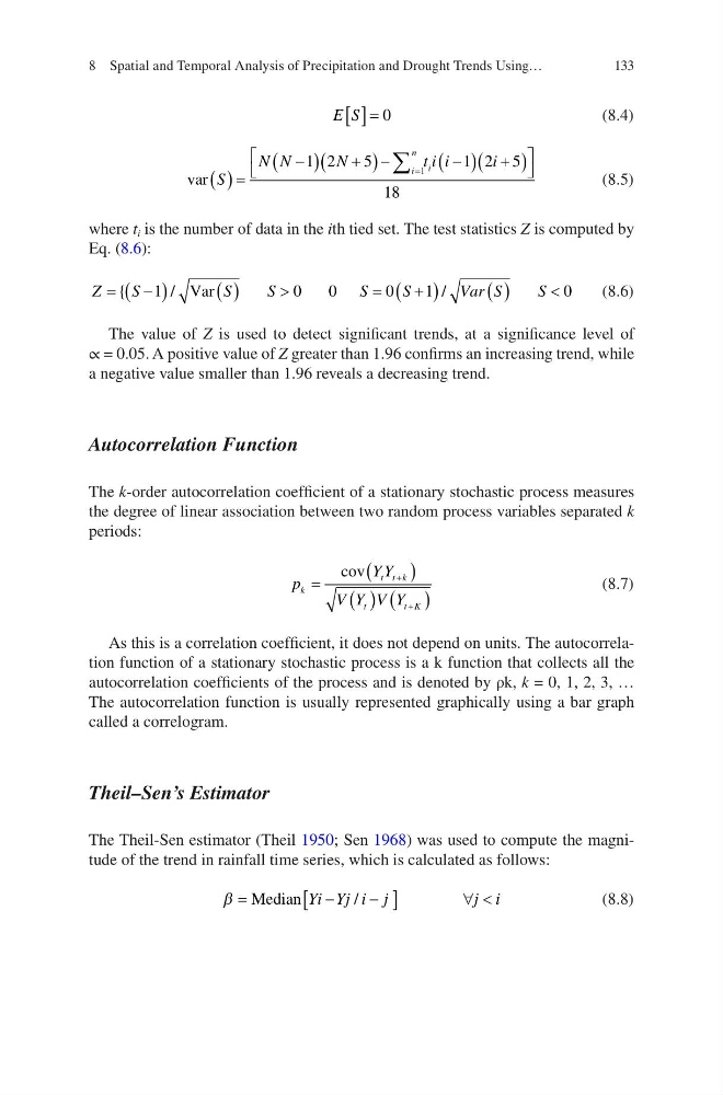
where t i is the number of data in the ith tied set. The test statistics Z is computed by
Eq. (8.6):
Z
S
S
S
S
S
Var S
S
=
-
( )
( )
>
=
+
( )
( )
<
{
/
/
1
0
0
0
1
0
Var
(8.6)
The value of Z is used to detect significant trends, at a significance level of
∝ = 0.05. A positive value of Z greater than 1.96 confirms an increasing trend, while
a negative value smaller than 1.96 reveals a decreasing trend.
Autocorrelation Function
The k-order autocorrelation coefficient of a stationary stochastic process measures
the degree of linear association between two random process variables separated k
periods:
p
Y Y
V Y V Y
k
t t k
t
t K
=
(
)
( ) ( )
+
+
cov
(8.7)
As this is a correlation coefficient, it does not depend on units. The autocorrelation function of a stationary stochastic process is a k function that collects all the
autocorrelation coefficients of the process and is denoted by ρk, k = 0, 1, 2, 3, …
The autocorrelation function is usually represented graphically using a bar graph
called a correlogram.
Theil–Sen’s Estimator
The Theil-Sen estimator (Theil 1950; Sen 1968) was used to compute the magnitude of the trend in rainfall time series, which is calculated as follows:
b =
-
-
[
]
" <
Median Yi Yj i j
j i
/
(8.8)
8 Spatial and Temporal Analysis of Precipitation and Drought Trends Using…
E S
[ ]= 0
(8.4)
var S
N N
N
ti i
i
i
n
i
( ) =
-
(
) +
(
-
( ) +
(
)
é
ë
ù
û
=
å
1 2
5
1 2 5
18
1
(8.5)
where t i is the number of data in the ith tied set. The test statistics Z is computed by
Eq. (8.6):
Z
S
S
S
S
S
Var S
S
=
-
( )
( )
>
=
+
( )
( )
<
{
/
/
1
0
0
0
1
0
Var
(8.6)
The value of Z is used to detect significant trends, at a significance level of
∝ = 0.05. A positive value of Z greater than 1.96 confirms an increasing trend, while
a negative value smaller than 1.96 reveals a decreasing trend.
Autocorrelation Function
The k-order autocorrelation coefficient of a stationary stochastic process measures
the degree of linear association between two random process variables separated k
periods:
p
Y Y
V Y V Y
k
t t k
t
t K
=
(
)
( ) ( )
+
+
cov
(8.7)
As this is a correlation coefficient, it does not depend on units. The autocorrelation function of a stationary stochastic process is a k function that collects all the
autocorrelation coefficients of the process and is denoted by ρk, k = 0, 1, 2, 3, …
The autocorrelation function is usually represented graphically using a bar graph
called a correlogram.
Theil–Sen’s Estimator
The Theil-Sen estimator (Theil 1950; Sen 1968) was used to compute the magnitude of the trend in rainfall time series, which is calculated as follows:
b =
-
-
[
]
" <
Median Yi Yj i j
j i
/
(8.8)
8 Spatial and Temporal Analysis of Precipitation and Drought Trends Using…