

Coarse-Grained Force Fields Built on Atomistic …
163
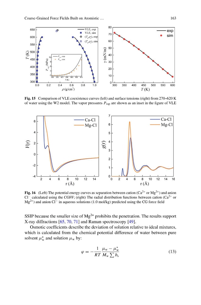
Fig. 15 Comparison of VLE coexistence curves (left) and surface tensions (right) from 270–620 K
of water using the W2 model. The vapor pressures P vap are shown as an inset in the figure of VLE
Fig. 16 (Left) The potential energy curves as separation between cation (Ca 2+ or Mg 2+ ) and anion
Cl − calculated using the CGFF; (right) The radial distribution functions between cation (Ca 2+ or
Mg 2+ ) and anion Cl − in aqueous solutions (1.0 mol/kg) predicted using the CG force field
SSIP because the smaller size of Mg
2+ prohibits the penetration. The results support
X-ray diffractions [65, 70, 71] and Raman spectroscopy [49].
Osmotic coefficients describe the deviation of solution relative to ideal mixtures,
which is calculated from the chemical potential difference of water between pure
solvent μ
∗
w and solution μ w by:
ϕ = −
1
RT
μ w − μ
∗
w
M w
b s
(13)
163
Fig. 15 Comparison of VLE coexistence curves (left) and surface tensions (right) from 270–620 K
of water using the W2 model. The vapor pressures P vap are shown as an inset in the figure of VLE
Fig. 16 (Left) The potential energy curves as separation between cation (Ca 2+ or Mg 2+ ) and anion
Cl − calculated using the CGFF; (right) The radial distribution functions between cation (Ca 2+ or
Mg 2+ ) and anion Cl − in aqueous solutions (1.0 mol/kg) predicted using the CG force field
SSIP because the smaller size of Mg
2+ prohibits the penetration. The results support
X-ray diffractions [65, 70, 71] and Raman spectroscopy [49].
Osmotic coefficients describe the deviation of solution relative to ideal mixtures,
which is calculated from the chemical potential difference of water between pure
solvent μ
∗
w and solution μ w by:
ϕ = −
1
RT
μ w − μ
∗
w
M w
b s
(13)