

164
H. Sun et al.
0.5
1.0
1.5
2.0
2.5
3.0
3.5
0.5
1.0
1.5
2.0
2.5
0.5
1.0
1.5
2.0
2.5
3.0
3.5
2
4
6
8
10
12
Osmotic Coefficient
Molality (mol/kg)
CaCl 2 , exp
CaCl 2 , sim
MgCl 2 , exp
MgCl 2 , sim
Surface Tension Increase (mN/m)
Molality (mol/kg)
CaCl 2 , exp
CaCl 2 , sim
MgCl 2 , exp
MgCl 2 , sim
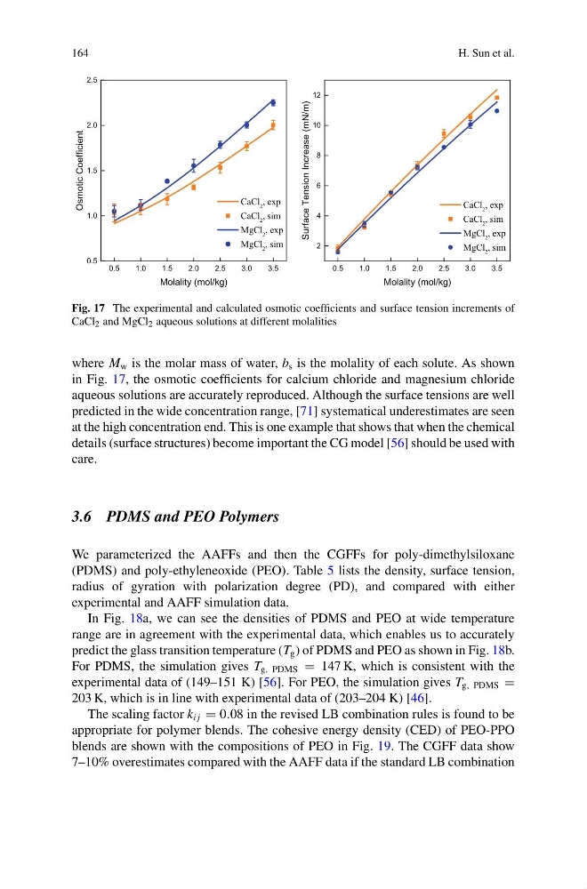
Fig. 17 The experimental and calculated osmotic coefficients and surface tension increments of
CaCl 2 and MgCl 2 aqueous solutions at different molalities
where M w is the molar mass of water, b s is the molality of each solute. As shown
in Fig. 17, the osmotic coefficients for calcium chloride and magnesium chloride
aqueous solutions are accurately reproduced. Although the surface tensions are well
predicted in the wide concentration range, [71] systematical underestimates are seen
at the high concentration end. This is one example that shows that when the chemical
details (surface structures) become important the CG model [56] should be used with
care.
3.6 PDMS and PEO Polymers
We parameterized the AAFFs and then the CGFFs for poly-dimethylsiloxane
(PDMS) and poly-ethyleneoxide (PEO). Table 5 lists the density, surface tension,
radius of gyration with polarization degree (PD), and compared with either
experimental and AAFF simulation data.
In Fig. 18a, we can see the densities of PDMS and PEO at wide temperature
range are in agreement with the experimental data, which enables us to accurately
predict the glass transition temperature (T g ) of PDMS and PEO as shown in Fig. 18b.
For PDMS, the simulation gives T g, PDMS = 147 K, which is consistent with the
experimental data of (149–151 K) [56]. For PEO, the simulation gives T g, PDMS =
203 K, which is in line with experimental data of (203–204 K) [46].
The scaling factor k i j = 0.08 in the revised LB combination rules is found to be
appropriate for polymer blends. The cohesive energy density (CED) of PEO-PPO
blends are shown with the compositions of PEO in Fig. 19. The CGFF data show
7–10% overestimates compared with the AAFF data if the standard LB combination
H. Sun et al.
0.5
1.0
1.5
2.0
2.5
3.0
3.5
0.5
1.0
1.5
2.0
2.5
0.5
1.0
1.5
2.0
2.5
3.0
3.5
2
4
6
8
10
12
Osmotic Coefficient
Molality (mol/kg)
CaCl 2 , exp
CaCl 2 , sim
MgCl 2 , exp
MgCl 2 , sim
Surface Tension Increase (mN/m)
Molality (mol/kg)
CaCl 2 , exp
CaCl 2 , sim
MgCl 2 , exp
MgCl 2 , sim
Fig. 17 The experimental and calculated osmotic coefficients and surface tension increments of
CaCl 2 and MgCl 2 aqueous solutions at different molalities
where M w is the molar mass of water, b s is the molality of each solute. As shown
in Fig. 17, the osmotic coefficients for calcium chloride and magnesium chloride
aqueous solutions are accurately reproduced. Although the surface tensions are well
predicted in the wide concentration range, [71] systematical underestimates are seen
at the high concentration end. This is one example that shows that when the chemical
details (surface structures) become important the CG model [56] should be used with
care.
3.6 PDMS and PEO Polymers
We parameterized the AAFFs and then the CGFFs for poly-dimethylsiloxane
(PDMS) and poly-ethyleneoxide (PEO). Table 5 lists the density, surface tension,
radius of gyration with polarization degree (PD), and compared with either
experimental and AAFF simulation data.
In Fig. 18a, we can see the densities of PDMS and PEO at wide temperature
range are in agreement with the experimental data, which enables us to accurately
predict the glass transition temperature (T g ) of PDMS and PEO as shown in Fig. 18b.
For PDMS, the simulation gives T g, PDMS = 147 K, which is consistent with the
experimental data of (149–151 K) [56]. For PEO, the simulation gives T g, PDMS =
203 K, which is in line with experimental data of (203–204 K) [46].
The scaling factor k i j = 0.08 in the revised LB combination rules is found to be
appropriate for polymer blends. The cohesive energy density (CED) of PEO-PPO
blends are shown with the compositions of PEO in Fig. 19. The CGFF data show
7–10% overestimates compared with the AAFF data if the standard LB combination