

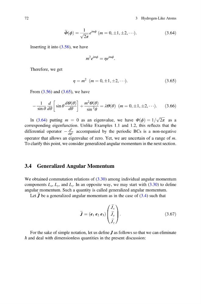
e
Φ ϕ
ð Þ ¼
1
ffiffiffiffiffi
2π
p e
imϕ m ¼ 0, Æ1, Æ2, Á Á Á
ð
Þ :
ð3:64Þ
Inserting it into (3.58), we have
m
2 e
imϕ
¼ ηe
imϕ
:
Therefore, we get
η ¼ m
2 m ¼ 0, Æ1, Æ2, Á Á Á
ð
Þ :
ð3:65Þ
From (3.56) and (3.65), we have
À
1
sin θ
d
dθ
sin θ
dΘ θ
ð Þ
dθ
!
þ
m
2
Θ θ
ð Þ
sin
2
θ
¼ λΘ θ
ð Þ m ¼ 0, Æ1, Æ2, Á Á Á
ð
Þ :
ð3:66Þ
In (3.64) putting m ¼ 0 as an eigenvalue, we have Φ ϕ
ð Þ ¼ 1=
ffiffiffiffiffi
2π
p
as a
corresponding eigenfunction. Unlike Examples 1.1 and 1.2, this reflects that the
differential operator À
d
2
dϕ
2 accompanied by the periodic BCs is a non-negative
operator that allows an eigenvalue of zero. Yet, we are uncertain of a range of m.
To clarify this point, we consider generalized angular momentum in the next section.
3.4 Generalized Angular Momentum
We obtained commutation relations of (3.30) among individual angular momentum
components L x , L y , and L z . In an opposite way, we may start with (3.30) to define
angular momentum. Such a quantity is called generalized angular momentum.
Let e J be a generalized angular momentum as in the case of (3.4) such that
e J ¼ e 1 e 2 e 3
ð
Þ
e
J x
e
J y
e
J z
0
B
@
1
C
A:
ð3:67Þ
For the sake of simple notation, let us define J as follows so that we can eliminate
ħ and deal with dimensionless quantities in the present discussion:
72
3 Hydrogen-Like Atoms
Φ ϕ
ð Þ ¼
1
ffiffiffiffiffi
2π
p e
imϕ m ¼ 0, Æ1, Æ2, Á Á Á
ð
Þ :
ð3:64Þ
Inserting it into (3.58), we have
m
2 e
imϕ
¼ ηe
imϕ
:
Therefore, we get
η ¼ m
2 m ¼ 0, Æ1, Æ2, Á Á Á
ð
Þ :
ð3:65Þ
From (3.56) and (3.65), we have
À
1
sin θ
d
dθ
sin θ
dΘ θ
ð Þ
dθ
!
þ
m
2
Θ θ
ð Þ
sin
2
θ
¼ λΘ θ
ð Þ m ¼ 0, Æ1, Æ2, Á Á Á
ð
Þ :
ð3:66Þ
In (3.64) putting m ¼ 0 as an eigenvalue, we have Φ ϕ
ð Þ ¼ 1=
ffiffiffiffiffi
2π
p
as a
corresponding eigenfunction. Unlike Examples 1.1 and 1.2, this reflects that the
differential operator À
d
2
dϕ
2 accompanied by the periodic BCs is a non-negative
operator that allows an eigenvalue of zero. Yet, we are uncertain of a range of m.
To clarify this point, we consider generalized angular momentum in the next section.
3.4 Generalized Angular Momentum
We obtained commutation relations of (3.30) among individual angular momentum
components L x , L y , and L z . In an opposite way, we may start with (3.30) to define
angular momentum. Such a quantity is called generalized angular momentum.
Let e J be a generalized angular momentum as in the case of (3.4) such that
e J ¼ e 1 e 2 e 3
ð
Þ
e
J x
e
J y
e
J z
0
B
@
1
C
A:
ð3:67Þ
For the sake of simple notation, let us define J as follows so that we can eliminate
ħ and deal with dimensionless quantities in the present discussion:
72
3 Hydrogen-Like Atoms