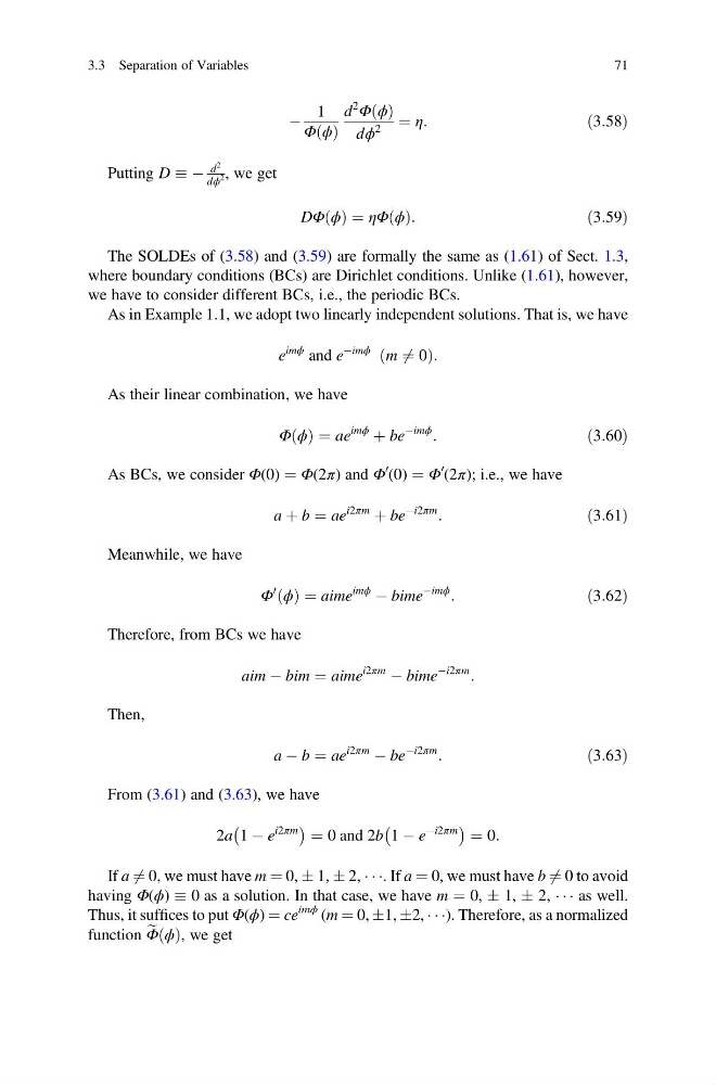
À
1
Φ ϕ
ð Þ
d
2
Φ ϕ
ð Þ
dϕ
2
¼ η:
ð3:58Þ
Putting D À
d
2
dϕ
2 , we get
DΦ ϕ
ð Þ ¼ ηΦ ϕ
ð Þ:
ð3:59Þ
The SOLDEs of (3.58) and (3.59) are formally the same as (1.61) of Sect. 1.3,
where boundary conditions (BCs) are Dirichlet conditions. Unlike (1.61), however,
we have to consider different BCs, i.e., the periodic BCs.
As in Example 1.1, we adopt two linearly independent solutions. That is, we have
e
imϕ and e
Àimϕ m 6 ¼ 0
ð
Þ:
As their linear combination, we have
Φ ϕ
ð Þ ¼ ae
imϕ
þ be
Àimϕ
:
ð3:60Þ
As BCs, we consider Φ(0) ¼ Φ(2π) and Φ
0 (0) ¼ Φ
0
(2π); i.e., we have
a þ b ¼ ae
i2πm
þ be
Ài2πm
:
ð3:61Þ
Meanwhile, we have
Φ
0
ϕ
ð Þ ¼ aime
imϕ
À bime
Àimϕ
:
ð3:62Þ
Therefore, from BCs we have
aim À bim ¼ aime
i2πm
À bime
Ài2πm
:
Then,
a À b ¼ ae
i2πm
À be
Ài2πm
:
ð3:63Þ
From (3.61) and (3.63), we have
2a 1 À e
i2πm
À
Á ¼ 0 and 2b 1 À e
Ài2πm
À
Á ¼ 0:
If a 6 ¼ 0, we must have m ¼ 0, Æ 1, Æ 2, Á Á Á. If a ¼ 0, we must have b 6 ¼ 0 to avoid
having Φ(ϕ) 0 as a solution. In that case, we have m ¼ 0, Æ 1, Æ 2, Á Á Á as well.
Thus, it suffices to put Φ(ϕ) ¼ ce
imϕ (m ¼ 0, Æ1, Æ2, Á Á Á). Therefore, as a normalized
function e
Φ ϕ
ð Þ, we get
3.3 Separation of Variables
71