

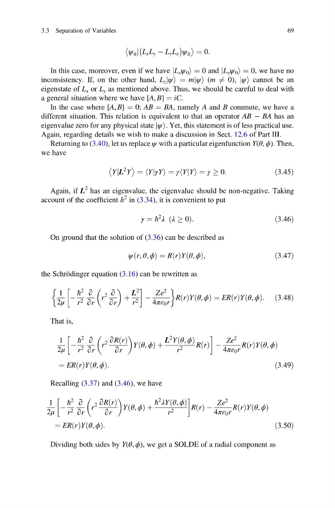
ψ 0 j L x L y À L y L x
À
Á ψ 0
¼ 0:
In this case, moreover, even if we have jL x ψ 0 i ¼ 0 and jL y ψ 0 i ¼ 0, we have no
inconsistency. If, on the other hand, L z jψi ¼ mjψi (m 6 ¼ 0), jψi cannot be an
eigenstate of L x or L y as mentioned above. Thus, we should be careful to deal with
a general situation where we have [A, B] ¼ iC.
In the case where [A, B] ¼ 0; AB ¼ BA, namely A and B commute, we have a
different situation. This relation is equivalent to that an operator AB À BA has an
eigenvalue zero for any physical state jψi. Yet, this statement is of less practical use.
Again, regarding details we wish to make a discussion in Sect. 12.6 of Part III.
Returning to (3.40), let us replace ψ with a particular eigenfunction Y(θ, ϕ). Then,
we have
YjL
2 Y
¼ YjγYi
h
¼ γ YjYi
h
¼ γ ! 0:
ð3:45Þ
Again, if L
2 has an eigenvalue, the eigenvalue should be non-negative. Taking
account of the coefficient ħ
2 in (3.34), it is convenient to put
γ ¼ ħ
2
λ λ ! 0
ð
Þ:
ð3:46Þ
On ground that the solution of (3.36) can be described as
ψ r, θ, ϕ
ð
Þ¼R r
ð ÞY θ, ϕ
ð
Þ,
ð3:47Þ
the Schrödinger equation (3.16) can be rewritten as
1
2μ
À
ħ
2
r 2
∂
∂r
r
2 ∂
∂r
þ
L
2
r 2
!
À
Ze
2
4πε 0 r
&
'
R r
ð ÞY θ, ϕ
ð
Þ ¼ ER r
ð ÞY θ, ϕ
ð
Þ: ð3:48Þ
That is,
1
2μ
À
ħ
2
r 2
∂
∂r
r
2 ∂R r
ð Þ
∂r
Y θ, ϕ
ð
Þþ
L
2 Y θ, ϕ
ð
Þ
r 2
R r
ð Þ
!
À
Ze
2
4πε 0 r
R r
ð ÞY θ, ϕ
ð
Þ
¼ ER r
ð ÞY θ, ϕ
ð
Þ:
ð3:49Þ
Recalling (3.37) and (3.46), we have
1
2μ
À
ħ
2
r 2
∂
∂r
r
2 ∂R r
ð Þ
∂r
Y θ, ϕ
ð
Þþ
ħ
2
λY θ, ϕ
ð
Þ
r 2
!
R r
ð Þ À
Ze
2
4πε 0 r
R r
ð ÞY θ, ϕ
ð
Þ
¼ ER r
ð ÞY θ, ϕ
ð
Þ:
ð3:50Þ
Dividing both sides by Y(θ, ϕ), we get a SOLDE of a radial component as
3.3 Separation of Variables
69
À
Á ψ 0
¼ 0:
In this case, moreover, even if we have jL x ψ 0 i ¼ 0 and jL y ψ 0 i ¼ 0, we have no
inconsistency. If, on the other hand, L z jψi ¼ mjψi (m 6 ¼ 0), jψi cannot be an
eigenstate of L x or L y as mentioned above. Thus, we should be careful to deal with
a general situation where we have [A, B] ¼ iC.
In the case where [A, B] ¼ 0; AB ¼ BA, namely A and B commute, we have a
different situation. This relation is equivalent to that an operator AB À BA has an
eigenvalue zero for any physical state jψi. Yet, this statement is of less practical use.
Again, regarding details we wish to make a discussion in Sect. 12.6 of Part III.
Returning to (3.40), let us replace ψ with a particular eigenfunction Y(θ, ϕ). Then,
we have
YjL
2 Y
¼ YjγYi
h
¼ γ YjYi
h
¼ γ ! 0:
ð3:45Þ
Again, if L
2 has an eigenvalue, the eigenvalue should be non-negative. Taking
account of the coefficient ħ
2 in (3.34), it is convenient to put
γ ¼ ħ
2
λ λ ! 0
ð
Þ:
ð3:46Þ
On ground that the solution of (3.36) can be described as
ψ r, θ, ϕ
ð
Þ¼R r
ð ÞY θ, ϕ
ð
Þ,
ð3:47Þ
the Schrödinger equation (3.16) can be rewritten as
1
2μ
À
ħ
2
r 2
∂
∂r
r
2 ∂
∂r
þ
L
2
r 2
!
À
Ze
2
4πε 0 r
&
'
R r
ð ÞY θ, ϕ
ð
Þ ¼ ER r
ð ÞY θ, ϕ
ð
Þ: ð3:48Þ
That is,
1
2μ
À
ħ
2
r 2
∂
∂r
r
2 ∂R r
ð Þ
∂r
Y θ, ϕ
ð
Þþ
L
2 Y θ, ϕ
ð
Þ
r 2
R r
ð Þ
!
À
Ze
2
4πε 0 r
R r
ð ÞY θ, ϕ
ð
Þ
¼ ER r
ð ÞY θ, ϕ
ð
Þ:
ð3:49Þ
Recalling (3.37) and (3.46), we have
1
2μ
À
ħ
2
r 2
∂
∂r
r
2 ∂R r
ð Þ
∂r
Y θ, ϕ
ð
Þþ
ħ
2
λY θ, ϕ
ð
Þ
r 2
!
R r
ð Þ À
Ze
2
4πε 0 r
R r
ð ÞY θ, ϕ
ð
Þ
¼ ER r
ð ÞY θ, ϕ
ð
Þ:
ð3:50Þ
Dividing both sides by Y(θ, ϕ), we get a SOLDE of a radial component as
3.3 Separation of Variables
69