

À
ħ
2
2μr 2
∂
∂r
r
2 ∂
∂r
þ
1
sinθ
∂
∂θ
sinθ
∂
∂θ
þ
1
sin
2
θ
∂
2
∂ϕ
2
"
#
À
Ze
2
4πε 0 r
(
)
ψ ¼Eψ: ð3:36Þ
3.3 Separation of Variables
If the potential is spherically symmetric (e.g., a Coulomb potential), it is well known
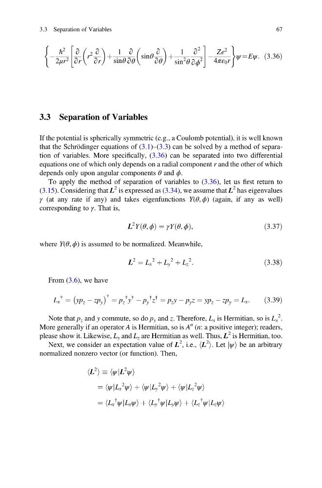
that the Schrödinger equations of (3.1)–(3.3) can be solved by a method of separation of variables. More specifically, (3.36) can be separated into two differential
equations one of which only depends on a radial component r and the other of which
depends only upon angular components θ and ϕ.
To apply the method of separation of variables to (3.36), let us first return to
(3.15). Considering that L
2 is expressed as (3.34), we assume that L
2 has eigenvalues
γ (at any rate if any) and takes eigenfunctions Y(θ, ϕ) (again, if any as well)
corresponding to γ. That is,
L
2 Y θ, ϕ
ð
Þ ¼ γY θ, ϕ
ð
Þ,
ð3:37Þ
where Y(θ, ϕ) is assumed to be normalized. Meanwhile,
L
2
¼ L x
2
þ L y
2
þ L z
2
:
ð3:38Þ
From (3.6), we have
L x
{
¼ yp z À zp y
À
Á { ¼ p z
{ y
{
À p y
{ z
{
¼ p z y À p y z ¼ yp z À zp y ¼ L x :
ð3:39Þ
Note that p z and y commute, so do p y and z. Therefore, L x is Hermitian, so is L x
2 .
More generally if an operator A is Hermitian, so is A
n (n: a positive integer); readers,
please show it. Likewise, L y and L z are Hermitian as well. Thus, L
2 is Hermitian, too.
Next, we consider an expectation value of L
2 , i.e., hL
2
i. Let jψi be an arbitrary
normalized nonzero vector (or function). Then,
hL
2
i hψ jL
2
ψi
¼ hψ jL x
2
ψi þ hψ jL y
2
ψi þ hψ jL z
2
ψi
¼ hL x
{
ψ jL x ψi þ hL y
{
ψ jL y ψi þ hL z
{
ψ jL z ψi
3.3 Separation of Variables
67
ħ
2
2μr 2
∂
∂r
r
2 ∂
∂r
þ
1
sinθ
∂
∂θ
sinθ
∂
∂θ
þ
1
sin
2
θ
∂
2
∂ϕ
2
"
#
À
Ze
2
4πε 0 r
(
)
ψ ¼Eψ: ð3:36Þ
3.3 Separation of Variables
If the potential is spherically symmetric (e.g., a Coulomb potential), it is well known
that the Schrödinger equations of (3.1)–(3.3) can be solved by a method of separation of variables. More specifically, (3.36) can be separated into two differential
equations one of which only depends on a radial component r and the other of which
depends only upon angular components θ and ϕ.
To apply the method of separation of variables to (3.36), let us first return to
(3.15). Considering that L
2 is expressed as (3.34), we assume that L
2 has eigenvalues
γ (at any rate if any) and takes eigenfunctions Y(θ, ϕ) (again, if any as well)
corresponding to γ. That is,
L
2 Y θ, ϕ
ð
Þ ¼ γY θ, ϕ
ð
Þ,
ð3:37Þ
where Y(θ, ϕ) is assumed to be normalized. Meanwhile,
L
2
¼ L x
2
þ L y
2
þ L z
2
:
ð3:38Þ
From (3.6), we have
L x
{
¼ yp z À zp y
À
Á { ¼ p z
{ y
{
À p y
{ z
{
¼ p z y À p y z ¼ yp z À zp y ¼ L x :
ð3:39Þ
Note that p z and y commute, so do p y and z. Therefore, L x is Hermitian, so is L x
2 .
More generally if an operator A is Hermitian, so is A
n (n: a positive integer); readers,
please show it. Likewise, L y and L z are Hermitian as well. Thus, L
2 is Hermitian, too.
Next, we consider an expectation value of L
2 , i.e., hL
2
i. Let jψi be an arbitrary
normalized nonzero vector (or function). Then,
hL
2
i hψ jL
2
ψi
¼ hψ jL x
2
ψi þ hψ jL y
2
ψi þ hψ jL z
2
ψi
¼ hL x
{
ψ jL x ψi þ hL y
{
ψ jL y ψi þ hL z
{
ψ jL z ψi
3.3 Separation of Variables
67