

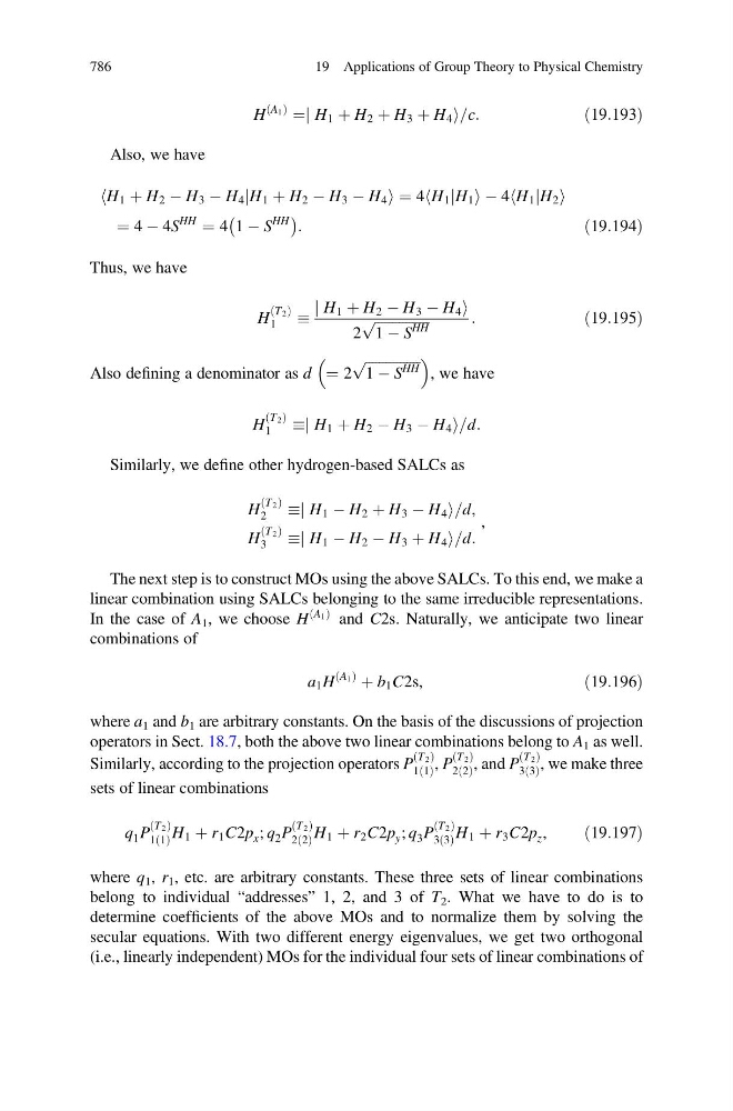
H
A 1
ð Þ
¼j H 1 þ H 2 þ H 3 þ H 4 i=c:
ð19:193Þ
Also, we have
H 1 þ H 2 À H 3 À H 4 jH 1 þ H 2 À H 3 À H 4
h
i ¼ 4 H 1 jH 1
h
iÀ 4 H 1 jH 2
h
i
¼ 4 À 4S
HH
¼ 4 1 À S
HH
À
Á :
ð19:194Þ
Thus, we have
H
T 2
ð Þ
1
j H 1 þ H 2 À H 3 À H 4 i
2
ffiffiffiffiffiffiffiffiffiffiffiffiffiffiffiffi
1 À S
HH
p
:
ð19:195Þ
Also defining a denominator as d ¼ 2
ffiffiffiffiffiffiffiffiffiffiffiffiffiffiffiffi
1 À S
HH
p
, we have
H
T 2
ð Þ
1
j H 1 þ H 2 À H 3 À H 4 i=d:
Similarly, we define other hydrogen-based SALCs as
H
T 2
ð Þ
2
j H 1 À H 2 þ H 3 À H 4 i=d,
H
T 2
ð Þ
3
j H 1 À H 2 À H 3 þ H 4 i=d:
,
The next step is to construct MOs using the above SALCs. To this end, we make a
linear combination using SALCs belonging to the same irreducible representations.
In the case of A 1 , we choose H
A 1
ð Þ and C2s. Naturally, we anticipate two linear
combinations of
a 1 H
A 1
ð Þ
þ b 1 C2s,
ð19:196Þ
where a 1 and b 1 are arbitrary constants. On the basis of the discussions of projection
operators in Sect. 18.7, both the above two linear combinations belong to A 1 as well.
Similarly, according to the projection operators P
T 2
ð Þ
1 1
ð Þ , P
T 2
ð Þ
2 2
ð Þ , and P
T 2
ð Þ
3 3
ð Þ , we make three
sets of linear combinations
q 1 P
T 2
ð Þ
1 1
ð Þ H 1 þ r 1 C2p x ; q 2 P
T 2
ð Þ
2 2
ð Þ H 1 þ r 2 C2p y ; q 3 P
T 2
ð Þ
3 3
ð Þ H 1 þ r 3 C2p z ,
ð19:197Þ
where q 1 , r 1 , etc. are arbitrary constants. These three sets of linear combinations
belong to individual “addresses” 1, 2, and 3 of T 2 . What we have to do is to
determine coefficients of the above MOs and to normalize them by solving the
secular equations. With two different energy eigenvalues, we get two orthogonal
(i.e., linearly independent) MOs for the individual four sets of linear combinations of
786
19 Applications of Group Theory to Physical Chemistry
A 1
ð Þ
¼j H 1 þ H 2 þ H 3 þ H 4 i=c:
ð19:193Þ
Also, we have
H 1 þ H 2 À H 3 À H 4 jH 1 þ H 2 À H 3 À H 4
h
i ¼ 4 H 1 jH 1
h
iÀ 4 H 1 jH 2
h
i
¼ 4 À 4S
HH
¼ 4 1 À S
HH
À
Á :
ð19:194Þ
Thus, we have
H
T 2
ð Þ
1
j H 1 þ H 2 À H 3 À H 4 i
2
ffiffiffiffiffiffiffiffiffiffiffiffiffiffiffiffi
1 À S
HH
p
:
ð19:195Þ
Also defining a denominator as d ¼ 2
ffiffiffiffiffiffiffiffiffiffiffiffiffiffiffiffi
1 À S
HH
p
, we have
H
T 2
ð Þ
1
j H 1 þ H 2 À H 3 À H 4 i=d:
Similarly, we define other hydrogen-based SALCs as
H
T 2
ð Þ
2
j H 1 À H 2 þ H 3 À H 4 i=d,
H
T 2
ð Þ
3
j H 1 À H 2 À H 3 þ H 4 i=d:
,
The next step is to construct MOs using the above SALCs. To this end, we make a
linear combination using SALCs belonging to the same irreducible representations.
In the case of A 1 , we choose H
A 1
ð Þ and C2s. Naturally, we anticipate two linear
combinations of
a 1 H
A 1
ð Þ
þ b 1 C2s,
ð19:196Þ
where a 1 and b 1 are arbitrary constants. On the basis of the discussions of projection
operators in Sect. 18.7, both the above two linear combinations belong to A 1 as well.
Similarly, according to the projection operators P
T 2
ð Þ
1 1
ð Þ , P
T 2
ð Þ
2 2
ð Þ , and P
T 2
ð Þ
3 3
ð Þ , we make three
sets of linear combinations
q 1 P
T 2
ð Þ
1 1
ð Þ H 1 þ r 1 C2p x ; q 2 P
T 2
ð Þ
2 2
ð Þ H 1 þ r 2 C2p y ; q 3 P
T 2
ð Þ
3 3
ð Þ H 1 þ r 3 C2p z ,
ð19:197Þ
where q 1 , r 1 , etc. are arbitrary constants. These three sets of linear combinations
belong to individual “addresses” 1, 2, and 3 of T 2 . What we have to do is to
determine coefficients of the above MOs and to normalize them by solving the
secular equations. With two different energy eigenvalues, we get two orthogonal
(i.e., linearly independent) MOs for the individual four sets of linear combinations of
786
19 Applications of Group Theory to Physical Chemistry