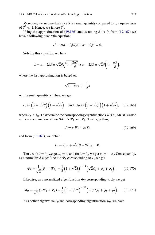
Moreover, we assume that since S is a small quantity compared to 1, a square term
of S
2
( 1. Hence, we ignore S
2 .
Using the approximation of (19.166) and assuming S
2
% 0, from (19.167) we
have a following quadratic equation:
λ
2
À 2 α À 2βS
ð
Þ λ þ α
2
À 2β
2
¼ 0:
Solving this equation, we have
λ ¼ α À 2βS Æ
ffiffi ffi
2
p β
ffiffiffiffiffiffiffiffiffiffiffiffiffiffiffiffi
1 À
2αS
β
r
% α À 2βS Æ
ffiffi ffi
2
p β 1 À
αS
β
,
where the last approximation is based on
ffiffiffiffiffiffiffiffiffiffi ffi
1 À x
p
% 1 À
1
2
x
with a small quantity x. Thus, we get
λ L % α þ
ffiffi ffi
2
p β
1 À
ffiffi ffi
2
p
S
and λ H % α À
ffiffi ffi
2
p β
1 þ
ffiffi ffi
2
p
S
, ð19:168Þ
where λ L < λ H . To determine the corresponding eigenfunctions Φ (i.e., MOs), we use
a linear combination of two SALCs Ψ 1 and Ψ 2 . That is, putting
Φ ¼ c 1 Ψ 1 þ c 2 Ψ 2
ð19:169Þ
and from (19.167), we obtain
α À λ
ð
Þc 1 þ
ffiffi ffi
2
p β À Sλ
ð
Þc 2 ¼ 0:
Thus, with λ ¼ λ L we get c 1 ¼ c 2 and for λ ¼ λ H we get c 1 ¼ À c 2 . Consequently,
as a normalized eigenfunction Φ L corresponding to λ L we get
Φ L ¼
1
ffiffi ffi
2
p Ψ 1 þ Ψ 2
ð
Þ¼
1
2
1 þ
ffiffi ffi
2
p
S
À1=2 ffiffi ffi
2
p ϕ 1 þ ϕ 2 þ ϕ 3
:
ð19:170Þ
Likewise, as a normalized eigenfunction Φ H corresponding to λ H we get
Φ H ¼
1
ffiffi ffi
2
p ÀΨ 1 þ Ψ 2
ð
Þ¼
1
2
1 À
ffiffi ffi
2
p
S
À1=2 À
ffiffi ffi
2
p ϕ 1 þ ϕ 2 þ ϕ 3
:
ð19:171Þ
As another eigenvalue λ 0 and corresponding eigenfunction Φ 0 , we have
19.4 MO Calculations Based on π-Electron Approximation
773