

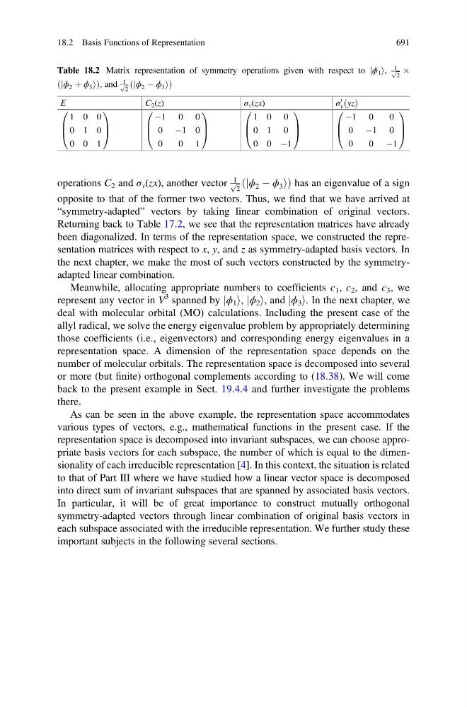
operations C 2 and σ v (zx), another vector
1 ffiffi
2
p jϕ 2 À ϕ 3 i
ð
Þhas an eigenvalue of a sign
opposite to that of the former two vectors. Thus, we find that we have arrived at
“symmetry-adapted” vectors by taking linear combination of original vectors.
Returning back to Table 17.2, we see that the representation matrices have already
been diagonalized. In terms of the representation space, we constructed the representation matrices with respect to x, y, and z as symmetry-adapted basis vectors. In
the next chapter, we make the most of such vectors constructed by the symmetryadapted linear combination.
Meanwhile, allocating appropriate numbers to coefficients c 1 , c 2 , and c 3 , we
represent any vector in V
3 spanned by jϕ 1 i, jϕ 2 i, and jϕ 3 i. In the next chapter, we
deal with molecular orbital (MO) calculations. Including the present case of the
allyl radical, we solve the energy eigenvalue problem by appropriately determining
those coefficients (i.e., eigenvectors) and corresponding energy eigenvalues in a
representation space. A dimension of the representation space depends on the
number of molecular orbitals. The representation space is decomposed into several
or more (but finite) orthogonal complements according to (18.38). We will come
back to the present example in Sect. 19.4.4 and further investigate the problems
there.
As can be seen in the above example, the representation space accommodates
various types of vectors, e.g., mathematical functions in the present case. If the
representation space is decomposed into invariant subspaces, we can choose appropriate basis vectors for each subspace, the number of which is equal to the dimensionality of each irreducible representation [4]. In this context, the situation is related
to that of Part III where we have studied how a linear vector space is decomposed
into direct sum of invariant subspaces that are spanned by associated basis vectors.
In particular, it will be of great importance to construct mutually orthogonal
symmetry-adapted vectors through linear combination of original basis vectors in
each subspace associated with the irreducible representation. We further study these
important subjects in the following several sections.
Table 18.2 Matrix representation of symmetry operations given with respect to jϕ 1 i,
1 ffiffi
2
p Â
jϕ 2 þ ϕ 3 i
ð
Þ , and
1 ffiffi
2
p jϕ 2 À ϕ 3 i
ð
Þ
E
C 2 (z)
σ v (zx)
σ
0
v yz
ð Þ
1 0 0
0 1 0
0 0 1
0
B
@
1
C
A
À1 0 0
0 À1 0
0
0 1
0
B
@
1
C
A
1 0 0
0 1 0
0 0 À1
0
B
@
1
C
A
À1 0
0
0 À1 0
0
0 À1
0
B
@
1
C
A
18.2 Basis Functions of Representation
691
1 ffiffi
2
p jϕ 2 À ϕ 3 i
ð
Þhas an eigenvalue of a sign
opposite to that of the former two vectors. Thus, we find that we have arrived at
“symmetry-adapted” vectors by taking linear combination of original vectors.
Returning back to Table 17.2, we see that the representation matrices have already
been diagonalized. In terms of the representation space, we constructed the representation matrices with respect to x, y, and z as symmetry-adapted basis vectors. In
the next chapter, we make the most of such vectors constructed by the symmetryadapted linear combination.
Meanwhile, allocating appropriate numbers to coefficients c 1 , c 2 , and c 3 , we
represent any vector in V
3 spanned by jϕ 1 i, jϕ 2 i, and jϕ 3 i. In the next chapter, we
deal with molecular orbital (MO) calculations. Including the present case of the
allyl radical, we solve the energy eigenvalue problem by appropriately determining
those coefficients (i.e., eigenvectors) and corresponding energy eigenvalues in a
representation space. A dimension of the representation space depends on the
number of molecular orbitals. The representation space is decomposed into several
or more (but finite) orthogonal complements according to (18.38). We will come
back to the present example in Sect. 19.4.4 and further investigate the problems
there.
As can be seen in the above example, the representation space accommodates
various types of vectors, e.g., mathematical functions in the present case. If the
representation space is decomposed into invariant subspaces, we can choose appropriate basis vectors for each subspace, the number of which is equal to the dimensionality of each irreducible representation [4]. In this context, the situation is related
to that of Part III where we have studied how a linear vector space is decomposed
into direct sum of invariant subspaces that are spanned by associated basis vectors.
In particular, it will be of great importance to construct mutually orthogonal
symmetry-adapted vectors through linear combination of original basis vectors in
each subspace associated with the irreducible representation. We further study these
important subjects in the following several sections.
Table 18.2 Matrix representation of symmetry operations given with respect to jϕ 1 i,
1 ffiffi
2
p Â
jϕ 2 þ ϕ 3 i
ð
Þ , and
1 ffiffi
2
p jϕ 2 À ϕ 3 i
ð
Þ
E
C 2 (z)
σ v (zx)
σ
0
v yz
ð Þ
1 0 0
0 1 0
0 0 1
0
B
@
1
C
A
À1 0 0
0 À1 0
0
0 1
0
B
@
1
C
A
1 0 0
0 1 0
0 0 À1
0
B
@
1
C
A
À1 0
0
0 À1 0
0
0 À1
0
B
@
1
C
A
18.2 Basis Functions of Representation
691