

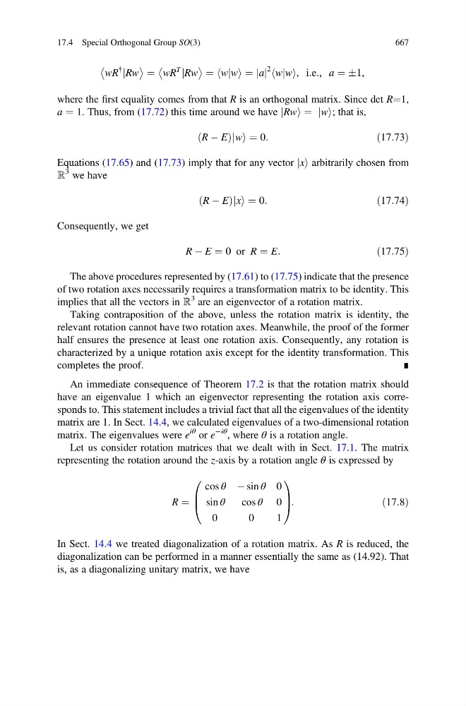
wR
{
jRw
¼ wR
T
jRw
¼ wjw
h
i ¼ a
j j
2 wjw
h
i, i:e:, a ¼ Æ1,
where the first equality comes from that R is an orthogonal matrix. Since det R¼1,
a ¼ 1. Thus, from (17.72) this time around we have jRwi ¼ jwi; that is,
R À E
ð
Þjwi ¼ 0:
ð17:73Þ
Equations (17.65) and (17.73) imply that for any vector jxi arbitrarily chosen from
ℝ
3 we have
R À E
ð
Þjxi ¼ 0:
ð17:74Þ
Consequently, we get
R À E ¼ 0 or R ¼ E:
ð17:75Þ
The above procedures represented by (17.61) to (17.75) indicate that the presence
of two rotation axes necessarily requires a transformation matrix to be identity. This
implies that all the vectors in ℝ
3 are an eigenvector of a rotation matrix.
Taking contraposition of the above, unless the rotation matrix is identity, the
relevant rotation cannot have two rotation axes. Meanwhile, the proof of the former
half ensures the presence at least one rotation axis. Consequently, any rotation is
characterized by a unique rotation axis except for the identity transformation. This
completes the proof.
∎
An immediate consequence of Theorem 17.2 is that the rotation matrix should
have an eigenvalue 1 which an eigenvector representing the rotation axis corresponds to. This statement includes a trivial fact that all the eigenvalues of the identity
matrix are 1. In Sect. 14.4, we calculated eigenvalues of a two-dimensional rotation
matrix. The eigenvalues were e
iθ or e
Àiθ , where θ is a rotation angle.
Let us consider rotation matrices that we dealt with in Sect. 17.1. The matrix
representing the rotation around the z-axis by a rotation angle θ is expressed by
R ¼
cos θ À sin θ 0
sin θ
cos θ 0
0
0
1
0
B
@
1
C
A:
ð17:8Þ
In Sect. 14.4 we treated diagonalization of a rotation matrix. As R is reduced, the
diagonalization can be performed in a manner essentially the same as (14.92). That
is, as a diagonalizing unitary matrix, we have
17.4 Special Orthogonal Group SO(3)
667