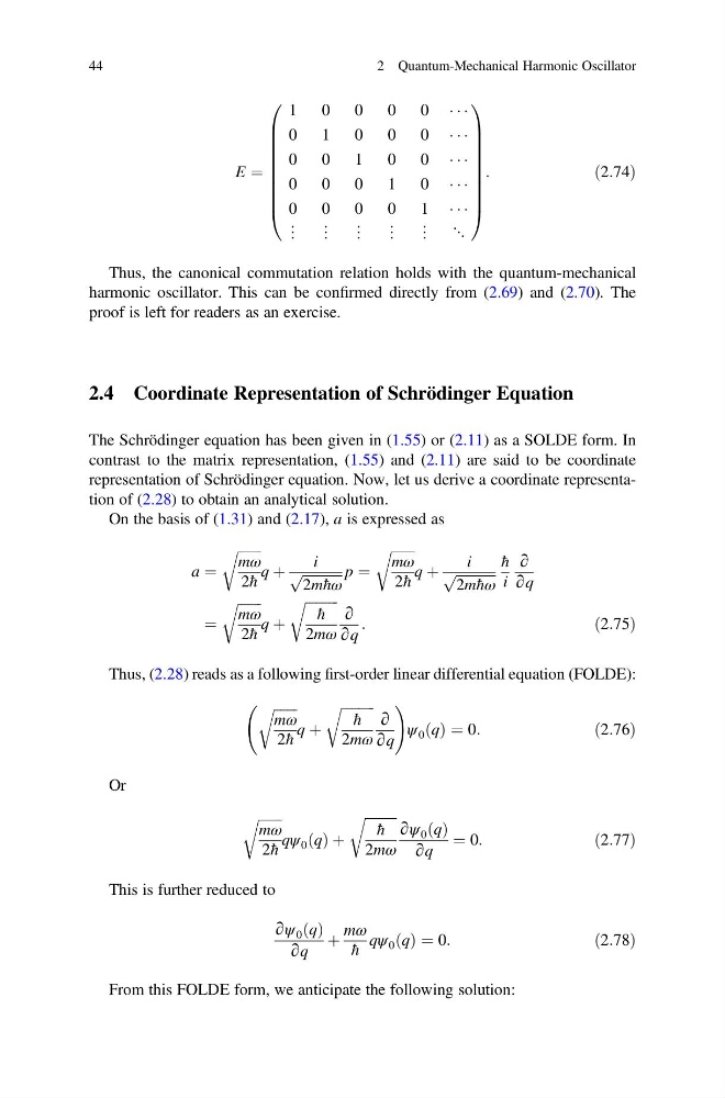
E ¼
1
0
0
0
0 Á Á Á
0
1
0
0
0 Á Á Á
0
0
1
0
0 Á Á Á
0
0
0
1
0 Á Á Á
0
0
0
0
1 Á Á Á
⋮ ⋮ ⋮ ⋮ ⋮ ⋱
0
B
B
B
B
B
B
B
B
@
1
C
C
C
C
C
C
C
C
A
:
ð2:74Þ
Thus, the canonical commutation relation holds with the quantum-mechanical
harmonic oscillator. This can be confirmed directly from (2.69) and (2.70). The
proof is left for readers as an exercise.
2.4 Coordinate Representation of Schrödinger Equation
The Schrödinger equation has been given in (1.55) or (2.11) as a SOLDE form. In
contrast to the matrix representation, (1.55) and (2.11) are said to be coordinate
representation of Schrödinger equation. Now, let us derive a coordinate representation of (2.28) to obtain an analytical solution.
On the basis of (1.31) and (2.17), a is expressed as
a ¼
ffiffiffiffiffiffiffi
mω
2ħ
r
q þ
i
ffiffiffiffiffiffiffiffiffiffiffiffi
2mħω
p
p ¼
ffiffiffiffiffiffiffi
mω
2ħ
r
q þ
i
ffiffiffiffiffiffiffiffiffiffiffiffi
2mħω
p
ħ
i
∂
∂q
¼
ffiffiffiffiffiffiffi
mω
2ħ
r
q þ
ffiffiffiffiffiffiffiffiffi ffi
ħ
2mω
r
∂
∂q
:
ð2:75Þ
Thus, (2.28) reads as a following first-order linear differential equation (FOLDE):
ffiffiffiffiffiffiffi
mω
2ħ
r
q þ
ffiffiffiffiffiffiffiffiffi ffi
ħ
2mω
r
∂
∂q
!
ψ 0 q
ð Þ ¼ 0:
ð2:76Þ
Or
ffiffiffiffiffiffiffi
mω
2ħ
r
qψ 0 q
ð Þ þ
ffiffiffiffiffiffiffiffiffi ffi
ħ
2mω
r
∂ψ 0 q
ð Þ
∂q
¼ 0:
ð2:77Þ
This is further reduced to
∂ψ 0 q
ð Þ
∂q
þ
mω
ħ
qψ 0 q
ð Þ ¼ 0:
ð2:78Þ
From this FOLDE form, we anticipate the following solution:
44
2 Quantum-Mechanical Harmonic Oscillator