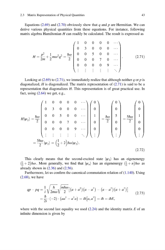
Equations (2.69) and (2.70) obviously show that q and p are Hermitian. We can
derive various physical quantities from these equations. For instance, following
matrix algebra Hamiltonian H can readily be calculated. The result is expressed as
H ¼
p
2
2m
þ
1
2
mω
2 q
2
¼
ħω
2
1 0
0
0
0 Á Á Á
0 3
0
0
0 Á Á Á
0 0
5
0
0 Á Á Á
0 0
0
7
0 Á Á Á
0 0
0
0
9 Á Á Á
⋮ ⋮ ⋮ ⋮ ⋮ ⋱
0
B
B
B
B
B
B
B
B
@
1
C
C
C
C
C
C
C
C
A
:
ð2:71Þ
Looking at (2.69) to (2.71), we immediately realize that although neither q or p is
diagonalized, H is diagonalized. The matrix representation of (2.71) is said to be a
representation that diagonalizes H. This representation is of great practical use. In
fact, using (2.64) we get, e.g.,
H ψ 2
j i ¼
ħω
2
1
0
0
0
0 Á Á Á
0
3
0
0
0 Á Á Á
0
0
5
0
0 Á Á Á
0
0
0
7
0 Á Á Á
0
0
0
0
9 Á Á Á
⋮ ⋮ ⋮ ⋮ ⋮ ⋱
0
B
B
B
B
B
B
B
B
B
B
B
@
1
C
C
C
C
C
C
C
C
C
C
C
A
0
0
1
0
0
⋮
0
B
B
B
B
B
B
B
B
B
B
B
@
1
C
C
C
C
C
C
C
C
C
C
C
A
¼
ħω
2
0
0
5
0
0
⋮
0
B
B
B
B
B
B
B
B
B
B
B
@
1
C
C
C
C
C
C
C
C
C
C
C
A
¼
5ħω
2
0
0
1
0
0
⋮
0
B
B
B
B
B
B
B
B
B
B
B
@
1
C
C
C
C
C
C
C
C
C
C
C
A
¼
5ħω
2
ψ 2
j i ¼
1
2
þ 2
ħω ψ 2
j i:
ð2:72Þ
This clearly means that the second-excited state jψ 2 i has an eigenenergy
1
2 þ 2
À
Á ħω . More generally, we find that jψ n i has an eigenenergy
1
2 þ n
À
Á ħω as
already shown in (2.36) and (2.56).
Furthermore, let us confirm the canonical commutation relation of (1.140). Using
(2.68), we have
qp À pq ¼
1
i
ffiffiffiffiffiffiffiffiffi ffi
ħ
2mω
r
ffiffiffiffiffiffiffiffiffi ffi
mħω
2
r
a þ a
{
À
Á
a À a
{
À
Á À a À a
{
À
Á
a þ a
{
À
Á
Â
Ã
¼
ħ
2i
Á À2
ð ÞÁ aa
{
À a
{ a
À
Á ¼ iħ a, a
{
Â
à ¼ iħ ¼ iħE,
ð2:73Þ
where with the second last equality we used (2.24) and the identity matrix E of an
infinite dimension is given by
2.3 Matrix Representation of Physical Quantities
43