

H a
{
À Á 2 j ψ 0 i ¼ E 0 þ 2ħω
ð
Þa
{
À Á 2 j ψ 0 i:
ð2:35Þ
This implies that (a
{ )
2
j ψ 0 i belongs to an eigenvalue (E 0 + 2ħω). Thus, repeatedly taking the above procedures, we get
H a
{
À Á n j ψ 0 i ¼ E 0 þ nħω
ð
Þa
{
À Á n j ψ 0 i:
ð2:36Þ
Thus, (a
{ )
n
j ψ 0 i belongs to an eigenvalue
E n E 0 þ nħω
ð
Þ¼ n þ
1
2
ħω,
ð2:37Þ
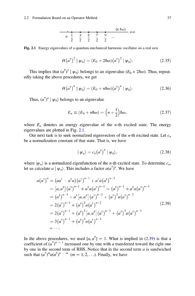
where E n denotes an energy eigenvalue of the n-th excited state. The energy
eigenvalues are plotted in Fig. 2.1.
Our next task is to seek normalized eigenvectors of the n-th excited state. Let c n
be a normalization constant of that state. That is, we have
j ψ n i ¼ c n a
{
À Á n j ψ 0 i,
ð2:38Þ
where jψ n i is a normalized eigenfunction of the n-th excited state. To determine c n ,
let us calculate a j ψ n i. This includes a factor a(a
{ )
n . We have
a a
{
À Á n ¼ aa
{
À a
{ a
À
Á
a
{
À Á nÀ1 þ a
{ a a
{
À Á nÀ1
¼ a, a
{
Â
Ã
a
{
À Á nÀ1 þ a
{ a a
{
À Á nÀ1 ¼ a
{
À Á nÀ1 þ a
{ a a
{
À Á nÀ1
¼ a
{
À Á nÀ1 þ a
{ a, a
{
Â
Ã
a
{
À Á nÀ2 þ a
{
À Á 2 a a
{
À Á nÀ2
¼ 2 a
{
À Á nÀ1 þ a
{
À Á 2 a a
{
À Á nÀ2
¼ 2 a
{
À Á nÀ1 þ a
{
À Á 2 a, a
{
Â
Ã
a
{
À Á nÀ3 þ a
{
À Á 3 a a
{
À Á nÀ3
¼ 3 a
{
À Á nÀ1 þ a
{
À Á 3 a a
{
À Á nÀ3
¼ Á Á Á:
ð2:39Þ
In the above procedures, we used [a, a
{ ] ¼ 1. What is implied in (2.39) is that a
coefficient of (a
{ )
n À 1 increased one by one with a transferred toward the right one
by one in the second term of RHS. Notice that in the second term a is sandwiched
such that (a
{ )
m
a(a
{ )
n À m (m ¼ 1, 2, . . .). Finally, we have
0
[ℏ +∞
⋯
1
2
3
2
5
2
7
2
9
2
Fig. 2.1 Energy eigenvalues of a quantum-mechanical harmonic oscillator on a real axis
2.2 Formulation Based on an Operator Method
37
{
À Á 2 j ψ 0 i ¼ E 0 þ 2ħω
ð
Þa
{
À Á 2 j ψ 0 i:
ð2:35Þ
This implies that (a
{ )
2
j ψ 0 i belongs to an eigenvalue (E 0 + 2ħω). Thus, repeatedly taking the above procedures, we get
H a
{
À Á n j ψ 0 i ¼ E 0 þ nħω
ð
Þa
{
À Á n j ψ 0 i:
ð2:36Þ
Thus, (a
{ )
n
j ψ 0 i belongs to an eigenvalue
E n E 0 þ nħω
ð
Þ¼ n þ
1
2
ħω,
ð2:37Þ
where E n denotes an energy eigenvalue of the n-th excited state. The energy
eigenvalues are plotted in Fig. 2.1.
Our next task is to seek normalized eigenvectors of the n-th excited state. Let c n
be a normalization constant of that state. That is, we have
j ψ n i ¼ c n a
{
À Á n j ψ 0 i,
ð2:38Þ
where jψ n i is a normalized eigenfunction of the n-th excited state. To determine c n ,
let us calculate a j ψ n i. This includes a factor a(a
{ )
n . We have
a a
{
À Á n ¼ aa
{
À a
{ a
À
Á
a
{
À Á nÀ1 þ a
{ a a
{
À Á nÀ1
¼ a, a
{
Â
Ã
a
{
À Á nÀ1 þ a
{ a a
{
À Á nÀ1 ¼ a
{
À Á nÀ1 þ a
{ a a
{
À Á nÀ1
¼ a
{
À Á nÀ1 þ a
{ a, a
{
Â
Ã
a
{
À Á nÀ2 þ a
{
À Á 2 a a
{
À Á nÀ2
¼ 2 a
{
À Á nÀ1 þ a
{
À Á 2 a a
{
À Á nÀ2
¼ 2 a
{
À Á nÀ1 þ a
{
À Á 2 a, a
{
Â
Ã
a
{
À Á nÀ3 þ a
{
À Á 3 a a
{
À Á nÀ3
¼ 3 a
{
À Á nÀ1 þ a
{
À Á 3 a a
{
À Á nÀ3
¼ Á Á Á:
ð2:39Þ
In the above procedures, we used [a, a
{ ] ¼ 1. What is implied in (2.39) is that a
coefficient of (a
{ )
n À 1 increased one by one with a transferred toward the right one
by one in the second term of RHS. Notice that in the second term a is sandwiched
such that (a
{ )
m
a(a
{ )
n À m (m ¼ 1, 2, . . .). Finally, we have
0
[ℏ +∞
⋯
1
2
3
2
5
2
7
2
9
2
Fig. 2.1 Energy eigenvalues of a quantum-mechanical harmonic oscillator on a real axis
2.2 Formulation Based on an Operator Method
37