

and that δ
j
k
ð Þ denotes a (1, n) matrix. Therefore, δ
k
ð Þ
i δ
j
k
ð Þ represents a (n, n) matrix
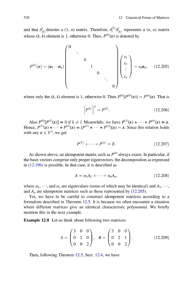
whose (k, k) element is 1, otherwise 0. Thus, P
(k)
(x) is denoted by
P
k
ð Þ x
ð Þ ¼ a 1 Á Á Áa n
ð
Þ
0
⋱
0
1
0
⋱
0
0
B
B
B
B
B
B
B
B
B
B
B
@
1
C
C
C
C
C
C
C
C
C
C
C
A
x 1
x 2
⋮
x n
0
B
B
B
@
1
C
C
C
A
¼ x k a k ,
ð12:205Þ
where only the (k, k) element is 1, otherwise 0. Then P
(k)
[P
(k) (x)] ¼ P
(k) (x). That is
P
k
ð Þ
h
i 2 ¼ P
k
ð Þ
:
ð12:206Þ
Also P
(k) [P
(l )
(x)] = 0 if k 6 ¼ l. Meanwhile, we have P
(1) (x) + Á Á Á + P
(n)
(x) = x.
Hence, P
(1) (x) + Á Á Á + P
(n)
(x) = [P
(1) + Á Á Á + P
(n) ](x) ¼ x. Since this relation holds
with any x 2 V
n , we get
P
1
ð Þ
þ Á Á Á þ P
n
ð Þ
¼ E:
ð12:207Þ
As shown above, an idempotent matrix such as P
(k) always exists. In particular, if
the basis vectors comprise only proper eigenvectors, the decomposition as expressed
in (12.196) is possible. In that case, it is described as
A ¼ α 1 A 1 þ Á Á Á þ α n A n ,
ð12:208Þ
where α 1 , Á Á Á, and α n are eigenvalues (some of which may be identical) and A 1 , Á Á Á,
and A n are idempotent matrices such as those represented by (12.205).
Yet, we have to be careful to construct idempotent matrices according to a
formalism described in Theorem 12.5. It is because we often encounter a situation
where different matrices give an identical characteristic polynomial. We briefly
mention this in the next example.
Example 12.8 Let us think about following two matrices:
A ¼
3 0 0
0 2 0
0 0 2
0
B
@
1
C
A, B ¼
3 0 0
0 2 1
0 0 2
0
B
@
1
C
A:
ð12:209Þ
Then, following Theorem 12.5, Sect. 12.4, we have
520
12 Canonical Forms of Matrices
j
k
ð Þ denotes a (1, n) matrix. Therefore, δ
k
ð Þ
i δ
j
k
ð Þ represents a (n, n) matrix
whose (k, k) element is 1, otherwise 0. Thus, P
(k)
(x) is denoted by
P
k
ð Þ x
ð Þ ¼ a 1 Á Á Áa n
ð
Þ
0
⋱
0
1
0
⋱
0
0
B
B
B
B
B
B
B
B
B
B
B
@
1
C
C
C
C
C
C
C
C
C
C
C
A
x 1
x 2
⋮
x n
0
B
B
B
@
1
C
C
C
A
¼ x k a k ,
ð12:205Þ
where only the (k, k) element is 1, otherwise 0. Then P
(k)
[P
(k) (x)] ¼ P
(k) (x). That is
P
k
ð Þ
h
i 2 ¼ P
k
ð Þ
:
ð12:206Þ
Also P
(k) [P
(l )
(x)] = 0 if k 6 ¼ l. Meanwhile, we have P
(1) (x) + Á Á Á + P
(n)
(x) = x.
Hence, P
(1) (x) + Á Á Á + P
(n)
(x) = [P
(1) + Á Á Á + P
(n) ](x) ¼ x. Since this relation holds
with any x 2 V
n , we get
P
1
ð Þ
þ Á Á Á þ P
n
ð Þ
¼ E:
ð12:207Þ
As shown above, an idempotent matrix such as P
(k) always exists. In particular, if
the basis vectors comprise only proper eigenvectors, the decomposition as expressed
in (12.196) is possible. In that case, it is described as
A ¼ α 1 A 1 þ Á Á Á þ α n A n ,
ð12:208Þ
where α 1 , Á Á Á, and α n are eigenvalues (some of which may be identical) and A 1 , Á Á Á,
and A n are idempotent matrices such as those represented by (12.205).
Yet, we have to be careful to construct idempotent matrices according to a
formalism described in Theorem 12.5. It is because we often encounter a situation
where different matrices give an identical characteristic polynomial. We briefly
mention this in the next example.
Example 12.8 Let us think about following two matrices:
A ¼
3 0 0
0 2 0
0 0 2
0
B
@
1
C
A, B ¼
3 0 0
0 2 1
0 0 2
0
B
@
1
C
A:
ð12:209Þ
Then, following Theorem 12.5, Sect. 12.4, we have
520
12 Canonical Forms of Matrices