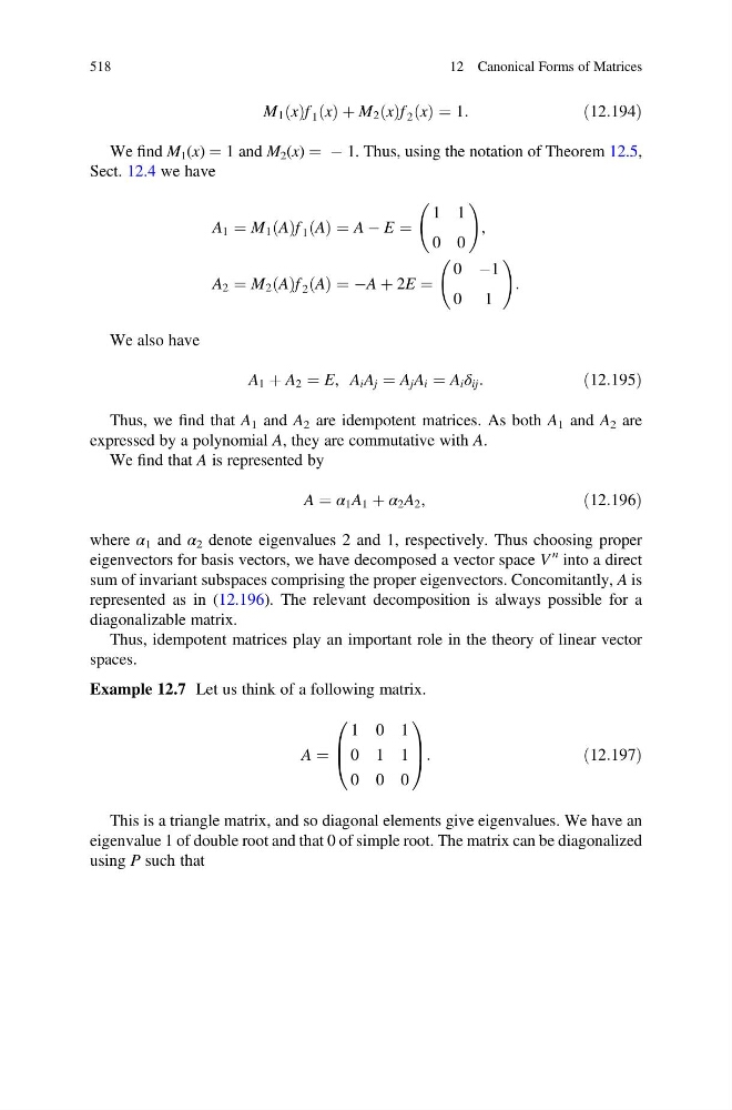
M 1 x
ð Þf 1 x
ð Þ þ M 2 x
ð Þf 2 x
ð Þ ¼ 1:
ð12:194Þ
We find M 1 (x) ¼ 1 and M 2 (x) ¼ À 1. Thus, using the notation of Theorem 12.5,
Sect. 12.4 we have
A 1 ¼ M 1 A
ð Þf 1 A
ð Þ ¼ A À E ¼
1 1
0 0
!
,
A 2 ¼ M 2 A
ð Þf 2 A
ð Þ ¼ ÀA þ 2E ¼
0 À1
0 1
!
:
We also have
A 1 þ A 2 ¼ E, A i A j ¼ A j A i ¼ A i δ ij :
ð12:195Þ
Thus, we find that A 1 and A 2 are idempotent matrices. As both A 1 and A 2 are
expressed by a polynomial A, they are commutative with A.
We find that A is represented by
A ¼ α 1 A 1 þ α 2 A 2 ,
ð12:196Þ
where α 1 and α 2 denote eigenvalues 2 and 1, respectively. Thus choosing proper
eigenvectors for basis vectors, we have decomposed a vector space V
n into a direct
sum of invariant subspaces comprising the proper eigenvectors. Concomitantly, A is
represented as in (12.196). The relevant decomposition is always possible for a
diagonalizable matrix.
Thus, idempotent matrices play an important role in the theory of linear vector
spaces.
Example 12.7 Let us think of a following matrix.
A ¼
1 0 1
0 1 1
0 0 0
0
B
@
1
C
A:
ð12:197Þ
This is a triangle matrix, and so diagonal elements give eigenvalues. We have an
eigenvalue 1 of double root and that 0 of simple root. The matrix can be diagonalized
using P such that
518
12 Canonical Forms of Matrices