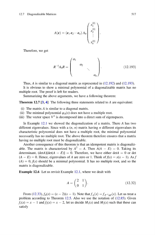
A x
ð Þ ¼ e 1 e 2 Á Á Áe n
ð
ÞA 0
x
0
ð Þ
1
x
0
ð Þ
2
⋮
x
0
ð Þ
n
0
B
B
B
B
@
1
C
C
C
C
A
:
Therefore, we get
R
À1 A 0 R ¼
α 1
α 2
⋱
α n
0
B
B
B
@
1
C
C
C
A
:
ð12:193Þ
Thus, A is similar to a diagonal matrix as represented in (12.192) and (12.193).
It is obvious to show a minimal polynomial of a diagonalizable matrix has no
multiple root. The proof is left for readers.
Summarizing the above arguments, we have a following theorem:
Theorem 12.7 [3, 4] The following three statements related to A are equivalent:
(i) The matrix A is similar to a diagonal matrix.
(ii) The minimal polynomial φ A (x) does not have a multiple root.
(iii) The vector space V
n is decomposed into a direct sum of eigenspaces.
In Example 12.1 we showed the diagonalization of a matrix. There A has two
different eigenvalues. Since with a (n, n) matrix having n different eigenvalues its
characteristic polynomial does not have a multiple root, the minimal polynomial
necessarily has no multiple root. The above theorem therefore ensures that a matrix
having no multiple root must be diagonalizable.
Another consequence of this theorem is that an idempotent matrix is diagonalizable. The matrix is characterized by A
2
¼ A. Then A(A À E) ¼ 0. Taking its
determinant, (detA)[det(A À E)] ¼ 0. Therefore, we have either detA ¼ 0 or det
(A À E) ¼ 0. Hence, eigenvalues of A are zero or 1. Think of f(x) ¼ x(x À 1). As f
(A) ¼ 0, f(x) should be a minimal polynomial. It has no multiple root, and so the
matrix is diagonalizable.
Example 12.6 Let us revisit Example 12.1, where we dealt with
A ¼
2 1
0 1
:
ð12:32Þ
From (12.33), f A (x) ¼ (x À 2)(x À 1). Note that f A x
ð Þ ¼ f P
À1 AP x
ð Þ. Let us treat a
problem according to Theorem 12.5. Also we use the notation of (12.85). Given
f 1 (x) ¼ x À 1 and f 2 (x) ¼ x À 2, let us decide M 1 (x) and M 2 (x) such that these can
satisfy
12.7 Diagonalizable Matrices
517