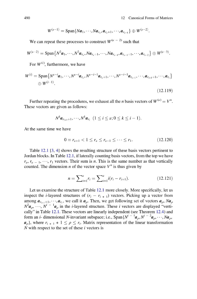
W
νÀ1
ð
Þ
¼ Span Na 1 , Á Á Á, Na r ν , a r ν þ1 , Á Á Á, a r νÀ1
f
g È W
νÀ2
ð
Þ
:
We can repeat these processes to construct W
(ν À 2) such that
W
νÀ2
ð
Þ
¼ Span N
2 a 1 , Á Á Á, N
2 a r ν , Na r ν þ1 , Á Á Á, Na r νÀ1 , a r νÀ1 þ1 , Á Á Á, a r νÀ2
È
É È W
νÀ3
ð
Þ
:
For W
(i)
, furthermore, we have
W
i
ð Þ
¼ Span N
νÀi a 1 , Á Á Á, N
νÀi a r ν , N
νÀiÀ1 a r ν þ1 , Á Á Á, N
νÀiÀ1 a r νÀ1 , Á Á Á, a r iþ1 þ1 , Á Á Á, a r i
È
É
È W
iÀ1
ð
Þ
:
ð12:119Þ
Further repeating the procedures, we exhaust all the n basis vectors of W
(ν) ¼ V
n .
These vectors are given as follows:
N
k a r iþ1 þ1 , Á Á Á, N
k a r i 1 i ν; 0 k i À 1
ð
Þ :
At the same time we have
0 r νþ1 < 1 r ν r νÀ1 Á Á Á r 1 :
ð12:120Þ
Table 12.1 [3, 4] shows the resulting structure of these basis vectors pertinent to
Jordan blocks. In Table 12.1, if laterally counting basis vectors, from the top we have
r ν , r ν À 1 , Á Á Á, r 1 vectors. Their sum is n. This is the same number as that vertically
counted. The dimension n of the vector space V
n is thus given by
n ¼
X ν
i¼1
r i ¼
X ν
i¼1
i r i À r iþ1
ð
Þ :
ð12:121Þ
Let us examine the structure of Table 12.1 more closely. More specifically, let us
inspect the i-layered structures of (r i À r i + 1 ) vectors. Picking up a vector from
among a r iþ1 þ1 , Á Á Á, a r i , we call it a ρ . Then, we get following set of vectors a ρ , Na ρ
N
2 a ρ , Á Á Á, N
i À 1 a ρ in the i-layered structure. These i vectors are displayed “vertically” in Table 12.1. These vectors are linearly independent (see Theorem 12.4) and
form an i- dimensional N-invariant subspace; i.e., Span{N
i À 1 a ρ , N
i À 2 a ρ , Á Á Á, Na ρ ,
a ρ }, where r i + 1 + 1 ρ r i . Matrix representation of the linear transformation
N with respect to the set of these i vectors is
490
12 Canonical Forms of Matrices