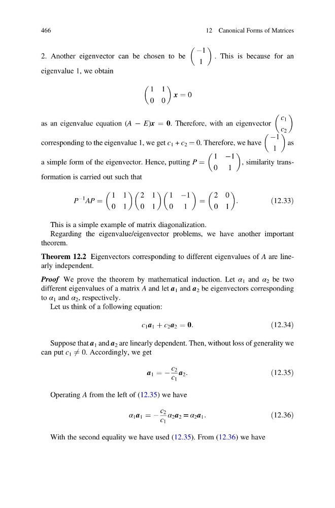
2. Another eigenvector can be chosen to be
À1
1
. This is because for an
eigenvalue 1, we obtain
1 1
0 0
x ¼ 0
as an eigenvalue equation (A À E)x ¼ 0. Therefore, with an eigenvector
c 1
c 2
corresponding to the eigenvalue 1, we get c 1 + c 2 ¼ 0. Therefore, we have
À1
1
as
a simple form of the eigenvector. Hence, putting P ¼
1 À1
0 1
, similarity transformation is carried out such that
P
À1 AP ¼
1 1
0 1
2 1
0 1
1 À1
0 1
¼
2 0
0 1
:
ð12:33Þ
This is a simple example of matrix diagonalization.
Regarding the eigenvalue/eigenvector problems, we have another important
theorem.
Theorem 12.2 Eigenvectors corresponding to different eigenvalues of A are linearly independent.
Proof We prove the theorem by mathematical induction. Let α 1 and α 2 be two
different eigenvalues of a matrix A and let a 1 and a 2 be eigenvectors corresponding
to α 1 and α 2 , respectively.
Let us think of a following equation:
c 1 a 1 þ c 2 a 2 ¼ 0:
ð12:34Þ
Suppose that a 1 and a 2 are linearly dependent. Then, without loss of generality we
can put c 1 6 ¼ 0. Accordingly, we get
a 1 ¼ À
c 2
c 1
a 2 :
ð12:35Þ
Operating A from the left of (12.35) we have
α 1 a 1 ¼ À
c 2
c 1
α 2 a 2 = α 2 a 1 :
ð12:36Þ
With the second equality we have used (12.35). From (12.36) we have
466
12 Canonical Forms of Matrices