

A x
ð Þ ¼ e 1 Á Á Áe n
ð
ÞPP
À1 A O PP
À1
x 1
⋮
x n
0
B
@
1
C
A:
ð11:83Þ
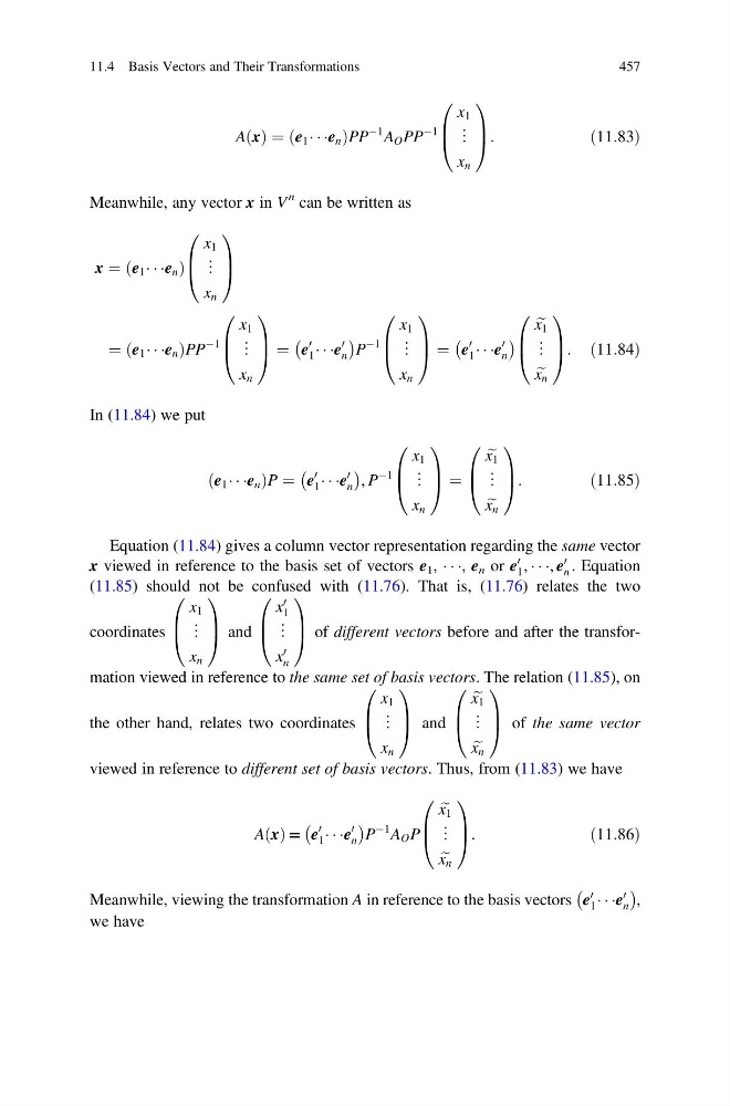
Meanwhile, any vector x in V
n can be written as
x ¼ e 1 Á Á Áe n
ð
Þ
x 1
⋮
x n
0
B
@
1
C
A
¼ e 1 Á Á Áe n
ð
ÞPP
À1
x 1
⋮
x n
0
B
@
1
C
A ¼ e
0
1 Á Á Áe
0
n
À
Á
P
À1
x 1
⋮
x n
0
B
@
1
C
A ¼ e
0
1 Á Á Áe
0
n
À
Á
e
x 1
⋮
e
x n
0
B
@
1
C
A: ð11:84Þ
In (11.84) we put
e 1 Á Á Áe n
ð
ÞP ¼ e
0
1 Á Á Áe
0
n
À
Á
, P
À1
x 1
⋮
x n
0
B
@
1
C
A ¼
e
x 1
⋮
e
x n
0
B
@
1
C
A:
ð11:85Þ
Equation (11.84) gives a column vector representation regarding the same vector
x viewed in reference to the basis set of vectors e 1 , Á Á Á, e n or e
0
1 , Á Á Á, e
0
n . Equation
(11.85) should not be confused with (11.76). That is, (11.76) relates the two
coordinates
x 1
⋮
x n
0
B
@
1
C
A and
x
0
1
⋮
x
0
n
0
B
@
1
C
A of different vectors before and after the transformation viewed in reference to the same set of basis vectors. The relation (11.85), on
the other hand, relates two coordinates
x 1
⋮
x n
0
B
@
1
C
A and
e
x 1
⋮
e
x n
0
B
@
1
C
A of the same vector
viewed in reference to different set of basis vectors. Thus, from (11.83) we have
A x
ð Þ = e
0
1 Á Á Áe
0
n
À
Á
P
À1 A O P
e
x 1
⋮
e
x n
0
B
@
1
C
A:
ð11:86Þ
Meanwhile, viewing the transformation A in reference to the basis vectors e
0
1 Á Á Áe
0
n
À
Á
,
we have
11.4 Basis Vectors and Their Transformations
457
ð Þ ¼ e 1 Á Á Áe n
ð
ÞPP
À1 A O PP
À1
x 1
⋮
x n
0
B
@
1
C
A:
ð11:83Þ
Meanwhile, any vector x in V
n can be written as
x ¼ e 1 Á Á Áe n
ð
Þ
x 1
⋮
x n
0
B
@
1
C
A
¼ e 1 Á Á Áe n
ð
ÞPP
À1
x 1
⋮
x n
0
B
@
1
C
A ¼ e
0
1 Á Á Áe
0
n
À
Á
P
À1
x 1
⋮
x n
0
B
@
1
C
A ¼ e
0
1 Á Á Áe
0
n
À
Á
e
x 1
⋮
e
x n
0
B
@
1
C
A: ð11:84Þ
In (11.84) we put
e 1 Á Á Áe n
ð
ÞP ¼ e
0
1 Á Á Áe
0
n
À
Á
, P
À1
x 1
⋮
x n
0
B
@
1
C
A ¼
e
x 1
⋮
e
x n
0
B
@
1
C
A:
ð11:85Þ
Equation (11.84) gives a column vector representation regarding the same vector
x viewed in reference to the basis set of vectors e 1 , Á Á Á, e n or e
0
1 , Á Á Á, e
0
n . Equation
(11.85) should not be confused with (11.76). That is, (11.76) relates the two
coordinates
x 1
⋮
x n
0
B
@
1
C
A and
x
0
1
⋮
x
0
n
0
B
@
1
C
A of different vectors before and after the transformation viewed in reference to the same set of basis vectors. The relation (11.85), on
the other hand, relates two coordinates
x 1
⋮
x n
0
B
@
1
C
A and
e
x 1
⋮
e
x n
0
B
@
1
C
A of the same vector
viewed in reference to different set of basis vectors. Thus, from (11.83) we have
A x
ð Þ = e
0
1 Á Á Áe
0
n
À
Á
P
À1 A O P
e
x 1
⋮
e
x n
0
B
@
1
C
A:
ð11:86Þ
Meanwhile, viewing the transformation A in reference to the basis vectors e
0
1 Á Á Áe
0
n
À
Á
,
we have
11.4 Basis Vectors and Their Transformations
457