

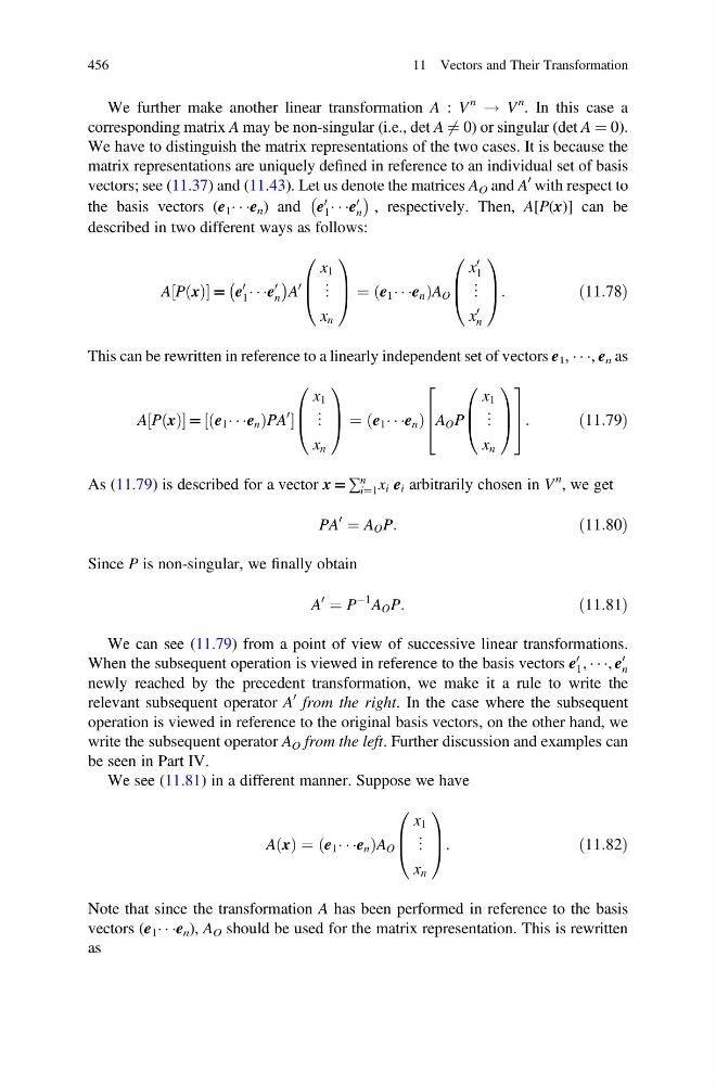
We further make another linear transformation A : V
n
! V
n . In this case a
corresponding matrix A may be non-singular (i.e., det A 6 ¼ 0) or singular (det A ¼ 0).
We have to distinguish the matrix representations of the two cases. It is because the
matrix representations are uniquely defined in reference to an individual set of basis
vectors; see (11.37) and (11.43). Let us denote the matrices A O and A
0 with respect to
the basis vectors (e 1 Á Á Áe n ) and e
0
1 Á Á Áe
0
n
À
Á
, respectively. Then, A[P(x)] can be
described in two different ways as follows:
A P x
ð Þ
½
= e
0
1 Á Á Áe
0
n
À
Á
A
0
x 1
⋮
x n
0
B
@
1
C
A ¼ e 1 Á Á Áe n
ð
ÞA O
x
0
1
⋮
x
0
n
0
B
@
1
C
A:
ð11:78Þ
This can be rewritten in reference to a linearly independent set of vectors e 1 , Á Á Á, e n as
A P x
ð Þ
½
= e 1 Á Á Áe n
ð
ÞPA
0
½
x 1
⋮
x n
0
B
@
1
C
A ¼ e 1 Á Á Áe n
ð
Þ A O P
x 1
⋮
x n
0
B
@
1
C
A
2
6
4
3
7
5:
ð11:79Þ
As (11.79) is described for a vector x = ∑
n
i¼1 x i e i arbitrarily chosen in V
n , we get
PA
0
¼ A O P:
ð11:80Þ
Since P is non-singular, we finally obtain
A
0
¼ P
À1 A O P:
ð11:81Þ
We can see (11.79) from a point of view of successive linear transformations.
When the subsequent operation is viewed in reference to the basis vectors e
0
1 , Á Á Á, e
0
n
newly reached by the precedent transformation, we make it a rule to write the
relevant subsequent operator A
0 from the right. In the case where the subsequent
operation is viewed in reference to the original basis vectors, on the other hand, we
write the subsequent operator A O from the left. Further discussion and examples can
be seen in Part IV.
We see (11.81) in a different manner. Suppose we have
A x
ð Þ ¼ e 1 Á Á Áe n
ð
ÞA O
x 1
⋮
x n
0
B
@
1
C
A:
ð11:82Þ
Note that since the transformation A has been performed in reference to the basis
vectors (e 1 Á Á Áe n ), A O should be used for the matrix representation. This is rewritten
as
456
11 Vectors and Their Transformation
n
! V
n . In this case a
corresponding matrix A may be non-singular (i.e., det A 6 ¼ 0) or singular (det A ¼ 0).
We have to distinguish the matrix representations of the two cases. It is because the
matrix representations are uniquely defined in reference to an individual set of basis
vectors; see (11.37) and (11.43). Let us denote the matrices A O and A
0 with respect to
the basis vectors (e 1 Á Á Áe n ) and e
0
1 Á Á Áe
0
n
À
Á
, respectively. Then, A[P(x)] can be
described in two different ways as follows:
A P x
ð Þ
½
= e
0
1 Á Á Áe
0
n
À
Á
A
0
x 1
⋮
x n
0
B
@
1
C
A ¼ e 1 Á Á Áe n
ð
ÞA O
x
0
1
⋮
x
0
n
0
B
@
1
C
A:
ð11:78Þ
This can be rewritten in reference to a linearly independent set of vectors e 1 , Á Á Á, e n as
A P x
ð Þ
½
= e 1 Á Á Áe n
ð
ÞPA
0
½
x 1
⋮
x n
0
B
@
1
C
A ¼ e 1 Á Á Áe n
ð
Þ A O P
x 1
⋮
x n
0
B
@
1
C
A
2
6
4
3
7
5:
ð11:79Þ
As (11.79) is described for a vector x = ∑
n
i¼1 x i e i arbitrarily chosen in V
n , we get
PA
0
¼ A O P:
ð11:80Þ
Since P is non-singular, we finally obtain
A
0
¼ P
À1 A O P:
ð11:81Þ
We can see (11.79) from a point of view of successive linear transformations.
When the subsequent operation is viewed in reference to the basis vectors e
0
1 , Á Á Á, e
0
n
newly reached by the precedent transformation, we make it a rule to write the
relevant subsequent operator A
0 from the right. In the case where the subsequent
operation is viewed in reference to the original basis vectors, on the other hand, we
write the subsequent operator A O from the left. Further discussion and examples can
be seen in Part IV.
We see (11.81) in a different manner. Suppose we have
A x
ð Þ ¼ e 1 Á Á Áe n
ð
ÞA O
x 1
⋮
x n
0
B
@
1
C
A:
ð11:82Þ
Note that since the transformation A has been performed in reference to the basis
vectors (e 1 Á Á Áe n ), A O should be used for the matrix representation. This is rewritten
as
456
11 Vectors and Their Transformation