

P x
ð Þ ¼ e 1 Á Á Áe n
ð
Þ
p 11 Á Á Á p 1n
⋮ ⋱ ⋮
p n1 Á Á Á p nn
0
B
@
1
C
A
x 1
⋮
x n
0
B
@
1
C
A,
ð11:73Þ
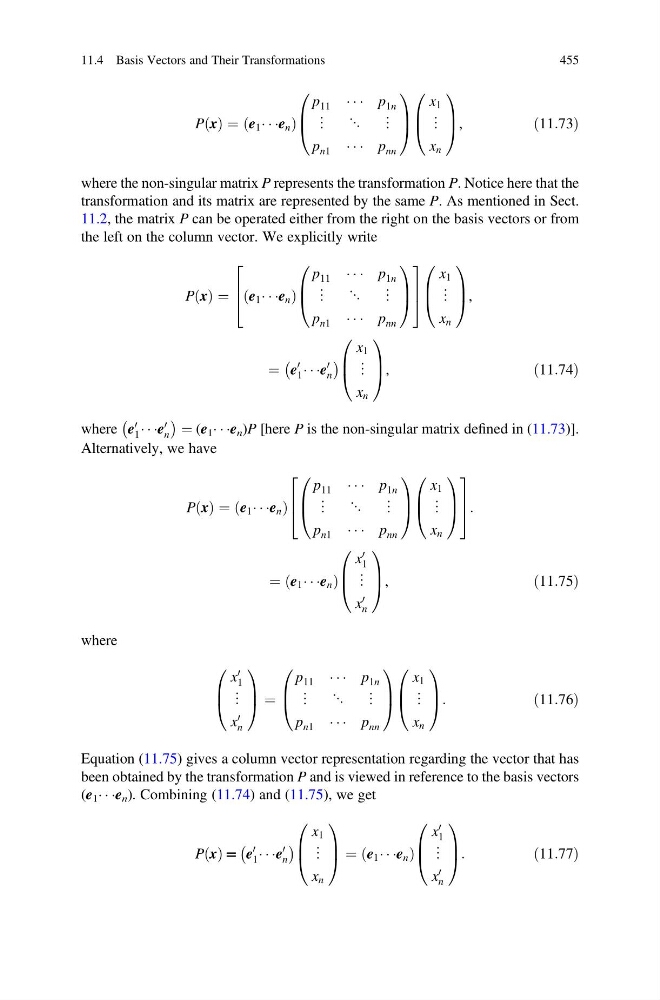
where the non-singular matrix P represents the transformation P. Notice here that the
transformation and its matrix are represented by the same P. As mentioned in Sect.
11.2, the matrix P can be operated either from the right on the basis vectors or from
the left on the column vector. We explicitly write
P x
ð Þ ¼ e 1 Á Á Áe n
ð
Þ
p 11 Á Á Á p 1n
⋮ ⋱ ⋮
p n1 Á Á Á p nn
0
B
@
1
C
A
2
6
4
3
7
5
x 1
⋮
x n
0
B
@
1
C
A,
¼ e
0
1 Á Á Áe
0
n
À
Á
x 1
⋮
x n
0
B
@
1
C
A,
ð11:74Þ
where e
0
1 Á Á Áe
0
n
À
Á ¼ (e 1 Á Á Áe n )P [here P is the non-singular matrix defined in (11.73)].
Alternatively, we have
P x
ð Þ ¼ e 1 Á Á Áe n
ð
Þ
p 11 Á Á Á p 1n
⋮ ⋱ ⋮
p n1 Á Á Á p nn
0
B
@
1
C
A
x 1
⋮
x n
0
B
@
1
C
A
2
6
4
3
7
5:
¼ e 1 Á Á Áe n
ð
Þ
x
0
1
⋮
x
0
n
0
B
@
1
C
A,
ð11:75Þ
where
x
0
1
⋮
x
0
n
0
B
@
1
C
A ¼
p 11 Á Á Á p 1n
⋮ ⋱ ⋮
p n1 Á Á Á p nn
0
B
@
1
C
A
x 1
⋮
x n
0
B
@
1
C
A:
ð11:76Þ
Equation (11.75) gives a column vector representation regarding the vector that has
been obtained by the transformation P and is viewed in reference to the basis vectors
(e 1 Á Á Áe n ). Combining (11.74) and (11.75), we get
P x
ð Þ = e
0
1 Á Á Áe
0
n
À
Á
x 1
⋮
x n
0
B
@
1
C
A ¼ e 1 Á Á Áe n
ð
Þ
x
0
1
⋮
x
0
n
0
B
@
1
C
A:
ð11:77Þ
11.4 Basis Vectors and Their Transformations
455
ð Þ ¼ e 1 Á Á Áe n
ð
Þ
p 11 Á Á Á p 1n
⋮ ⋱ ⋮
p n1 Á Á Á p nn
0
B
@
1
C
A
x 1
⋮
x n
0
B
@
1
C
A,
ð11:73Þ
where the non-singular matrix P represents the transformation P. Notice here that the
transformation and its matrix are represented by the same P. As mentioned in Sect.
11.2, the matrix P can be operated either from the right on the basis vectors or from
the left on the column vector. We explicitly write
P x
ð Þ ¼ e 1 Á Á Áe n
ð
Þ
p 11 Á Á Á p 1n
⋮ ⋱ ⋮
p n1 Á Á Á p nn
0
B
@
1
C
A
2
6
4
3
7
5
x 1
⋮
x n
0
B
@
1
C
A,
¼ e
0
1 Á Á Áe
0
n
À
Á
x 1
⋮
x n
0
B
@
1
C
A,
ð11:74Þ
where e
0
1 Á Á Áe
0
n
À
Á ¼ (e 1 Á Á Áe n )P [here P is the non-singular matrix defined in (11.73)].
Alternatively, we have
P x
ð Þ ¼ e 1 Á Á Áe n
ð
Þ
p 11 Á Á Á p 1n
⋮ ⋱ ⋮
p n1 Á Á Á p nn
0
B
@
1
C
A
x 1
⋮
x n
0
B
@
1
C
A
2
6
4
3
7
5:
¼ e 1 Á Á Áe n
ð
Þ
x
0
1
⋮
x
0
n
0
B
@
1
C
A,
ð11:75Þ
where
x
0
1
⋮
x
0
n
0
B
@
1
C
A ¼
p 11 Á Á Á p 1n
⋮ ⋱ ⋮
p n1 Á Á Á p nn
0
B
@
1
C
A
x 1
⋮
x n
0
B
@
1
C
A:
ð11:76Þ
Equation (11.75) gives a column vector representation regarding the vector that has
been obtained by the transformation P and is viewed in reference to the basis vectors
(e 1 Á Á Áe n ). Combining (11.74) and (11.75), we get
P x
ð Þ = e
0
1 Á Á Áe
0
n
À
Á
x 1
⋮
x n
0
B
@
1
C
A ¼ e 1 Á Á Áe n
ð
Þ
x
0
1
⋮
x
0
n
0
B
@
1
C
A:
ð11:77Þ
11.4 Basis Vectors and Their Transformations
455