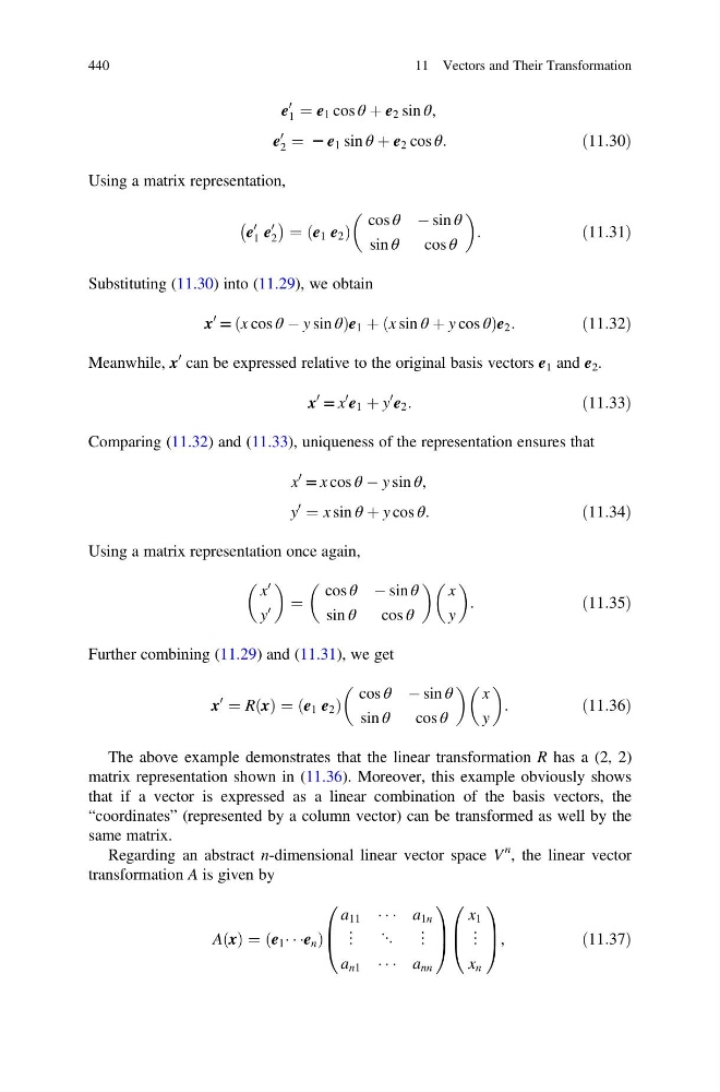
e
0
1 ¼ e 1 cos θ þ e 2 sin θ,
e
0
2 ¼ 2 e 1 sin θ þ e 2 cos θ:
ð11:30Þ
Using a matrix representation,
e
0
1 e
0
2
À
Á ¼ e 1 e 2
ð
Þ
cos θ À sin θ
sin θ
cos θ
:
ð11:31Þ
Substituting (11.30) into (11.29), we obtain
x
0
= x cos θ À y sin θ
ð
Þ e 1 þ x sin θ þ y cos θ
ð
Þ e 2 :
ð11:32Þ
Meanwhile, x
0 can be expressed relative to the original basis vectors e 1 and e 2 .
x
0
= x
0
e 1 þ y
0
e 2 :
ð11:33Þ
Comparing (11.32) and (11.33), uniqueness of the representation ensures that
x
0
= x cos θ À y sin θ,
y
0
¼ x sin θ þ y cos θ:
ð11:34Þ
Using a matrix representation once again,
x
0
y
0
¼
cos θ À sin θ
sin θ
cos θ
x
y
:
ð11:35Þ
Further combining (11.29) and (11.31), we get
x
0
¼ R x
ð Þ ¼ e 1 e 2
ð
Þ
cos θ À sin θ
sin θ
cos θ
x
y
:
ð11:36Þ
The above example demonstrates that the linear transformation R has a (2, 2)
matrix representation shown in (11.36). Moreover, this example obviously shows
that if a vector is expressed as a linear combination of the basis vectors, the
“coordinates” (represented by a column vector) can be transformed as well by the
same matrix.
Regarding an abstract n-dimensional linear vector space V
n , the linear vector
transformation A is given by
A x
ð Þ ¼ e 1 Á Á Áe n
ð
Þ
a 11 Á Á Á a 1n
⋮ ⋱ ⋮
a n1 Á Á Á a nn
0
B
@
1
C
A
x 1
⋮
x n
0
B
@
1
C
A,
ð11:37Þ
440
11 Vectors and Their Transformation