

where e 1 , e 2 , Á Á Á, and e n are basis vectors and x 1 , x 2 , Á Á Á, and x n are the corresponding
coordinates of a vector x = ∑
n
i¼1 x i e i . We assume that the transformation is a mapping
A: V
n
! V
n (i.e., endomorphism). In this case the transformation is represented by a
(n, n) matrix. Note that the matrix operates on the basis vectors from the right and
that it operates on the coordinates (i.e., a column vector) from the left. In (11.37) we
often omit a parenthesis to simply write Ax.
Here we mention matrix notation for later convenience. We often identify a linear
vector transformation with its representation matrix and denote both transformation
and matrix by A. On this occasion, we write
A ¼
a 11 Á Á Á a 1n
⋮ ⋱ ⋮
a n1 Á Á Á a nn
0
B
@
1
C
A, A ¼ A
ð Þ ij ¼ a ij
À Á
, etc:,
ð11:38Þ
where with the second expression (A) ij and (a ij ) represent the matrix A itself; for we
frequently use indexed matrix notations such as A
À1
, A
{ and e
A. The notation (11.38)
can conveniently be used in such cases. Note moreover that a ij represents the matrix
A as well.
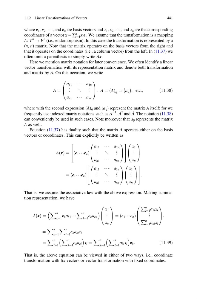
Equation (11.37) has duality such that the matrix A operates either on the basis
vectors or coordinates. This can explicitly be written as
A x
ð Þ ¼ e 1 Á Á Áe n
ð
Þ
a 11 Á Á Á a 1n
⋮ ⋱ ⋮
a n1 Á Á Á a nn
0
B
@
1
C
A
2
6
4
3
7
5
x 1
⋮
x n
0
B
@
1
C
A
¼ e 1 Á Á Áe n
ð
Þ
a 11 Á Á Á a 1n
⋮ ⋱ ⋮
a n1 Á Á Á a nn
0
B
@
1
C
A
x 1
⋮
x n
0
B
@
1
C
A
2
6
4
3
7
5:
That is, we assume the associative law with the above expression. Making summation representation, we have
A x
ð Þ ¼
X n
k¼1
e k a k1 Á Á Á
X n
k¼1
e k a kn
x 1
⋮
x n
0
B
@
1
C
A ¼ e 1 Á Á Áe n
ð
Þ
P n
l¼1 a 1l x l
⋮
P n
l¼1 a nl x l
0
B
@
1
C
A:
¼
X n
k¼1
X n
l¼1
e k a kl x l
¼
X n
l¼1
X n
k¼1
e k a kl
x l ¼
X n
k¼1
X n
l¼1
a kl x l
e k :
ð11:39Þ
That is, the above equation can be viewed in either of two ways, i.e., coordinate
transformation with fix vectors or vector transformation with fixed coordinates.
11.2 Linear Transformations of Vectors
441
coordinates of a vector x = ∑
n
i¼1 x i e i . We assume that the transformation is a mapping
A: V
n
! V
n (i.e., endomorphism). In this case the transformation is represented by a
(n, n) matrix. Note that the matrix operates on the basis vectors from the right and
that it operates on the coordinates (i.e., a column vector) from the left. In (11.37) we
often omit a parenthesis to simply write Ax.
Here we mention matrix notation for later convenience. We often identify a linear
vector transformation with its representation matrix and denote both transformation
and matrix by A. On this occasion, we write
A ¼
a 11 Á Á Á a 1n
⋮ ⋱ ⋮
a n1 Á Á Á a nn
0
B
@
1
C
A, A ¼ A
ð Þ ij ¼ a ij
À Á
, etc:,
ð11:38Þ
where with the second expression (A) ij and (a ij ) represent the matrix A itself; for we
frequently use indexed matrix notations such as A
À1
, A
{ and e
A. The notation (11.38)
can conveniently be used in such cases. Note moreover that a ij represents the matrix
A as well.
Equation (11.37) has duality such that the matrix A operates either on the basis
vectors or coordinates. This can explicitly be written as
A x
ð Þ ¼ e 1 Á Á Áe n
ð
Þ
a 11 Á Á Á a 1n
⋮ ⋱ ⋮
a n1 Á Á Á a nn
0
B
@
1
C
A
2
6
4
3
7
5
x 1
⋮
x n
0
B
@
1
C
A
¼ e 1 Á Á Áe n
ð
Þ
a 11 Á Á Á a 1n
⋮ ⋱ ⋮
a n1 Á Á Á a nn
0
B
@
1
C
A
x 1
⋮
x n
0
B
@
1
C
A
2
6
4
3
7
5:
That is, we assume the associative law with the above expression. Making summation representation, we have
A x
ð Þ ¼
X n
k¼1
e k a k1 Á Á Á
X n
k¼1
e k a kn
x 1
⋮
x n
0
B
@
1
C
A ¼ e 1 Á Á Áe n
ð
Þ
P n
l¼1 a 1l x l
⋮
P n
l¼1 a nl x l
0
B
@
1
C
A:
¼
X n
k¼1
X n
l¼1
e k a kl x l
¼
X n
l¼1
X n
k¼1
e k a kl
x l ¼
X n
k¼1
X n
l¼1
a kl x l
e k :
ð11:39Þ
That is, the above equation can be viewed in either of two ways, i.e., coordinate
transformation with fix vectors or vector transformation with fixed coordinates.
11.2 Linear Transformations of Vectors
441