

A ca þ db
ð
Þ= cA a
ð Þ þ dA b
ð Þ:
ð11:25Þ
We will briefly discuss the concepts of mapping at the end of this section.
It is convenient to define addition of the linear transformations. It is defined as
A þ B
ð
Þa = Aa þ Ba,
ð11:26Þ
where a is any vector in V.
Since (11.25) is a broad but abstract definition, we begin with a well-known
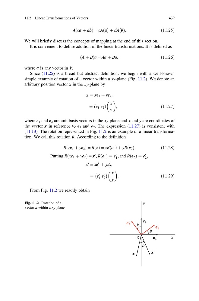
simple example of rotation of a vector within a xy-plane (Fig. 11.2). We denote an
arbitrary position vector x in the xy-plane by
x ¼ xe 1 þ ye 2 :
¼ e 1 e 2
ð
Þ
x
y
,
ð11:27Þ
where e 1 and e 2 are unit basis vectors in the xy-plane and x and y are coordinates of
the vector x in reference to e 1 and e 2 . The expression (11.27) is consistent with
(11.13). The rotation represented in Fig. 11.2 is an example of a linear transformation. We call this rotation R. According to the definition
R xe 1 þ ye 2
ð
Þ= R x
ð Þ = xR e 1
ð Þ þ yR e 2
ð Þ:
ð11:28Þ
Putting R xe 1 þ ye 2
ð
Þ= x
0 , R e 1
ð Þ ¼ e
0
1 , and R e 2
ð Þ ¼ e
0
2 ,
x
0
= xe
0
1 þ ye
0
2 ,
¼ e
0
1 e
0
2
À
Á x
y
:
ð11:29Þ
From Fig. 11.2 we readily obtain
θ
θ
′
θ
Fig. 11.2 Rotation of a
vector x within a xy-plane
11.2 Linear Transformations of Vectors
439
ð
Þ= cA a
ð Þ þ dA b
ð Þ:
ð11:25Þ
We will briefly discuss the concepts of mapping at the end of this section.
It is convenient to define addition of the linear transformations. It is defined as
A þ B
ð
Þa = Aa þ Ba,
ð11:26Þ
where a is any vector in V.
Since (11.25) is a broad but abstract definition, we begin with a well-known
simple example of rotation of a vector within a xy-plane (Fig. 11.2). We denote an
arbitrary position vector x in the xy-plane by
x ¼ xe 1 þ ye 2 :
¼ e 1 e 2
ð
Þ
x
y
,
ð11:27Þ
where e 1 and e 2 are unit basis vectors in the xy-plane and x and y are coordinates of
the vector x in reference to e 1 and e 2 . The expression (11.27) is consistent with
(11.13). The rotation represented in Fig. 11.2 is an example of a linear transformation. We call this rotation R. According to the definition
R xe 1 þ ye 2
ð
Þ= R x
ð Þ = xR e 1
ð Þ þ yR e 2
ð Þ:
ð11:28Þ
Putting R xe 1 þ ye 2
ð
Þ= x
0 , R e 1
ð Þ ¼ e
0
1 , and R e 2
ð Þ ¼ e
0
2 ,
x
0
= xe
0
1 þ ye
0
2 ,
¼ e
0
1 e
0
2
À
Á x
y
:
ð11:29Þ
From Fig. 11.2 we readily obtain
θ
θ
′
θ
Fig. 11.2 Rotation of a
vector x within a xy-plane
11.2 Linear Transformations of Vectors
439