

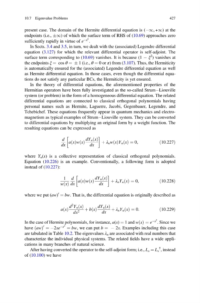
present case. The domain of the Hermite differential equation is (À1, +1) at the
endpoints (i.e., Æ1) of which the surface term of RHS of (10.69) approaches zero
sufficiently rapidly in virtue of e
Àx
2 .
In Sects. 3.4 and 3.5, in turn, we dealt with the (associated) Legendre differential
equation (3.127) for which the relevant differential operator is self-adjoint. The
surface term corresponding to (10.69) vanishes. It is because (1 À ξ
2 ) vanishes at
the endpoints ξ ¼ cos θ ¼ Æ 1 (i.e., θ ¼ 0 or π) from (3.107). Thus, the Hermiticity
is automatically ensured for the (associated) Legendre differential equation as well
as Hermite differential equation. In those cases, even though the differential equations do not satisfy any particular BCs, the Hermiticity is yet ensured.
In the theory of differential equations, the aforementioned properties of the
Hermitian operators have been fully investigated as the so-called StrumÀLiouville
system (or problem) in the form of a homogeneous differential equation. The related
differential equations are connected to classical orthogonal polynomials having
personal names such as Hermite, Laguerre, Jacobi, Gegenbauer, Legendre, and
Tchebichef. These equations frequently appear in quantum mechanics and electromagnetism as typical examples of StrumÀLiouville system. They can be converted
to differential equations by multiplying an original form by a weight function. The
resulting equations can be expressed as
d
dx
a x
ð Þw x
ð Þ
dY n x
ð Þ
dx
!
þ λ n w x
ð ÞY n x
ð Þ ¼ 0,
ð10:227Þ
where Y n (x) is a collective representation of classical orthogonal polynomials.
Equation (10.226) is an example. Conventionally, a following form is adopted
instead of (10.227):
1
w x
ð Þ
d
dx
a x
ð Þw x
ð Þ
dY n x
ð Þ
dx
!
þ λ n Y n x
ð Þ ¼ 0,
ð10:228Þ
where we put (aw)
0
¼ bw. That is, the differential equation is originally described as
a x
ð Þ
d
2 Y n x
ð Þ
dx 2 þ b x
ð Þ
dY n x
ð Þ
dx
þ λ n Y n x
ð Þ ¼ 0:
ð10:229Þ
In the case of Hermite polynomials, for instance, a(x) ¼ 1 and w x
ð Þ ¼ e
Àx
2 . Since we
have aw
ð Þ
0 ¼ À2xe
Àx
2 ¼ bw, we can put b ¼ À 2x. Examples including this case
are tabulated in Table 10.2. The eigenvalues λ n are associated with real numbers that
characterize the individual physical systems. The related fields have a wide applications in many branches of natural science.
After having converted the operator to the self-adjoint form; i.e., L x ¼ L x
{ , instead
of (10.100) we have
10.7 Eigenvalue Problems
427
endpoints (i.e., Æ1) of which the surface term of RHS of (10.69) approaches zero
sufficiently rapidly in virtue of e
Àx
2 .
In Sects. 3.4 and 3.5, in turn, we dealt with the (associated) Legendre differential
equation (3.127) for which the relevant differential operator is self-adjoint. The
surface term corresponding to (10.69) vanishes. It is because (1 À ξ
2 ) vanishes at
the endpoints ξ ¼ cos θ ¼ Æ 1 (i.e., θ ¼ 0 or π) from (3.107). Thus, the Hermiticity
is automatically ensured for the (associated) Legendre differential equation as well
as Hermite differential equation. In those cases, even though the differential equations do not satisfy any particular BCs, the Hermiticity is yet ensured.
In the theory of differential equations, the aforementioned properties of the
Hermitian operators have been fully investigated as the so-called StrumÀLiouville
system (or problem) in the form of a homogeneous differential equation. The related
differential equations are connected to classical orthogonal polynomials having
personal names such as Hermite, Laguerre, Jacobi, Gegenbauer, Legendre, and
Tchebichef. These equations frequently appear in quantum mechanics and electromagnetism as typical examples of StrumÀLiouville system. They can be converted
to differential equations by multiplying an original form by a weight function. The
resulting equations can be expressed as
d
dx
a x
ð Þw x
ð Þ
dY n x
ð Þ
dx
!
þ λ n w x
ð ÞY n x
ð Þ ¼ 0,
ð10:227Þ
where Y n (x) is a collective representation of classical orthogonal polynomials.
Equation (10.226) is an example. Conventionally, a following form is adopted
instead of (10.227):
1
w x
ð Þ
d
dx
a x
ð Þw x
ð Þ
dY n x
ð Þ
dx
!
þ λ n Y n x
ð Þ ¼ 0,
ð10:228Þ
where we put (aw)
0
¼ bw. That is, the differential equation is originally described as
a x
ð Þ
d
2 Y n x
ð Þ
dx 2 þ b x
ð Þ
dY n x
ð Þ
dx
þ λ n Y n x
ð Þ ¼ 0:
ð10:229Þ
In the case of Hermite polynomials, for instance, a(x) ¼ 1 and w x
ð Þ ¼ e
Àx
2 . Since we
have aw
ð Þ
0 ¼ À2xe
Àx
2 ¼ bw, we can put b ¼ À 2x. Examples including this case
are tabulated in Table 10.2. The eigenvalues λ n are associated with real numbers that
characterize the individual physical systems. The related fields have a wide applications in many branches of natural science.
After having converted the operator to the self-adjoint form; i.e., L x ¼ L x
{ , instead
of (10.100) we have
10.7 Eigenvalue Problems
427