

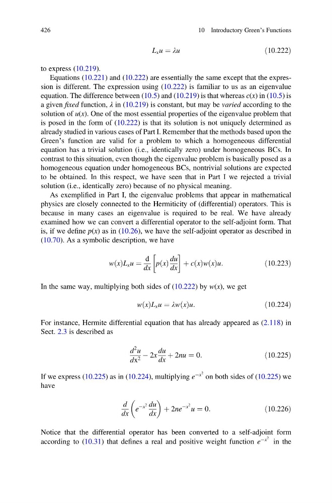
L x u ¼ λu
ð10:222Þ
to express (10.219).
Equations (10.221) and (10.222) are essentially the same except that the expression is different. The expression using (10.222) is familiar to us as an eigenvalue
equation. The difference between (10.5) and (10.219) is that whereas c(x) in (10.5) is
a given fixed function, λ in (10.219) is constant, but may be varied according to the
solution of u(x). One of the most essential properties of the eigenvalue problem that
is posed in the form of (10.222) is that its solution is not uniquely determined as
already studied in various cases of Part I. Remember that the methods based upon the
Green’s function are valid for a problem to which a homogeneous differential
equation has a trivial solution (i.e., identically zero) under homogeneous BCs. In
contrast to this situation, even though the eigenvalue problem is basically posed as a
homogeneous equation under homogeneous BCs, nontrivial solutions are expected
to be obtained. In this respect, we have seen that in Part I we rejected a trivial
solution (i.e., identically zero) because of no physical meaning.
As exemplified in Part I, the eigenvalue problems that appear in mathematical
physics are closely connected to the Hermiticity of (differential) operators. This is
because in many cases an eigenvalue is required to be real. We have already
examined how we can convert a differential operator to the self-adjoint form. That
is, if we define p(x) as in (10.26), we have the self-adjoint operator as described in
(10.70). As a symbolic description, we have
w x
ð ÞL x u ¼
d
dx
p x
ð Þ
du
dx
!
þ c x
ð Þw x
ð Þu:
ð10:223Þ
In the same way, multiplying both sides of (10.222) by w(x), we get
w x
ð ÞL x u ¼ λw x
ð Þu:
ð10:224Þ
For instance, Hermite differential equation that has already appeared as (2.118) in
Sect. 2.3 is described as
d
2 u
dx 2 À 2x
du
dx
þ 2nu ¼ 0:
ð10:225Þ
If we express (10.225) as in (10.224), multiplying e
Àx
2 on both sides of (10.225) we
have
d
dx
e
Àx
2 du
dx
þ 2ne
Àx
2 u ¼ 0:
ð10:226Þ
Notice that the differential operator has been converted to a self-adjoint form
according to (10.31) that defines a real and positive weight function e
Àx
2 in the
426
10 Introductory Green’s Functions
ð10:222Þ
to express (10.219).
Equations (10.221) and (10.222) are essentially the same except that the expression is different. The expression using (10.222) is familiar to us as an eigenvalue
equation. The difference between (10.5) and (10.219) is that whereas c(x) in (10.5) is
a given fixed function, λ in (10.219) is constant, but may be varied according to the
solution of u(x). One of the most essential properties of the eigenvalue problem that
is posed in the form of (10.222) is that its solution is not uniquely determined as
already studied in various cases of Part I. Remember that the methods based upon the
Green’s function are valid for a problem to which a homogeneous differential
equation has a trivial solution (i.e., identically zero) under homogeneous BCs. In
contrast to this situation, even though the eigenvalue problem is basically posed as a
homogeneous equation under homogeneous BCs, nontrivial solutions are expected
to be obtained. In this respect, we have seen that in Part I we rejected a trivial
solution (i.e., identically zero) because of no physical meaning.
As exemplified in Part I, the eigenvalue problems that appear in mathematical
physics are closely connected to the Hermiticity of (differential) operators. This is
because in many cases an eigenvalue is required to be real. We have already
examined how we can convert a differential operator to the self-adjoint form. That
is, if we define p(x) as in (10.26), we have the self-adjoint operator as described in
(10.70). As a symbolic description, we have
w x
ð ÞL x u ¼
d
dx
p x
ð Þ
du
dx
!
þ c x
ð Þw x
ð Þu:
ð10:223Þ
In the same way, multiplying both sides of (10.222) by w(x), we get
w x
ð ÞL x u ¼ λw x
ð Þu:
ð10:224Þ
For instance, Hermite differential equation that has already appeared as (2.118) in
Sect. 2.3 is described as
d
2 u
dx 2 À 2x
du
dx
þ 2nu ¼ 0:
ð10:225Þ
If we express (10.225) as in (10.224), multiplying e
Àx
2 on both sides of (10.225) we
have
d
dx
e
Àx
2 du
dx
þ 2ne
Àx
2 u ¼ 0:
ð10:226Þ
Notice that the differential operator has been converted to a self-adjoint form
according to (10.31) that defines a real and positive weight function e
Àx
2 in the
426
10 Introductory Green’s Functions