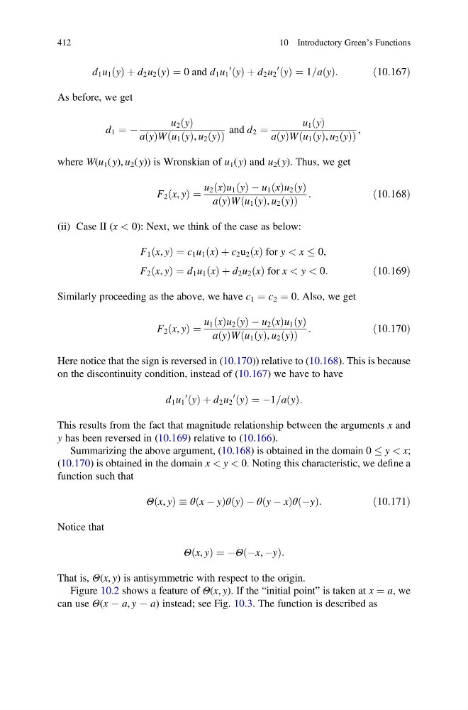
d 1 u 1 y
ð Þ þ d 2 u 2 y
ð Þ ¼ 0 and d 1 u 1
0 y
ð Þ þ d 2 u 2
0 y
ð Þ ¼ 1=a y
ð Þ:
ð10:167Þ
As before, we get
d 1 ¼ À
u 2 y
ð Þ
a y
ð ÞW u 1 y
ð Þ, u 2 y
ð Þ
ð
Þ
and d 2 ¼
u 1 y
ð Þ
a y
ð ÞW u 1 y
ð Þ, u 2 y
ð Þ
ð
Þ
,
where W(u 1 ( y), u 2 ( y)) is Wronskian of u 1 ( y) and u 2 ( y). Thus, we get
F 2 x, y
ð Þ ¼
u 2 x
ð Þu 1 y
ð Þ À u 1 x
ð Þu 2 y
ð Þ
a y
ð ÞW u 1 y
ð Þ, u 2 y
ð Þ
ð
Þ
:
ð10:168Þ
(ii) Case II (x < 0): Next, we think of the case as below:
F 1 x, y
ð Þ ¼ c 1 u 1 x
ð Þ þ c 2 u 2 x
ð Þ for y < x 0,
F 2 x, y
ð Þ ¼ d 1 u 1 x
ð Þ þ d 2 u 2 x
ð Þ for x < y < 0:
ð10:169Þ
Similarly proceeding as the above, we have c 1 ¼ c 2 ¼ 0. Also, we get
F 2 x, y
ð Þ ¼
u 1 x
ð Þu 2 y
ð Þ À u 2 x
ð Þu 1 y
ð Þ
a y
ð ÞW u 1 y
ð Þ, u 2 y
ð Þ
ð
Þ
:
ð10:170Þ
Here notice that the sign is reversed in (10.170)) relative to (10.168). This is because
on the discontinuity condition, instead of (10.167) we have to have
d 1 u 1
0 y
ð Þ þ d 2 u 2
0 y
ð Þ ¼ À1=a y
ð Þ:
This results from the fact that magnitude relationship between the arguments x and
y has been reversed in (10.169) relative to (10.166).
Summarizing the above argument, (10.168) is obtained in the domain 0 y < x;
(10.170) is obtained in the domain x < y < 0. Noting this characteristic, we define a
function such that
Θ x, y
ð Þ θ x À y
ð
Þθ y
ð Þ À θ y À x
ð
Þθ Ày
ð Þ:
ð10:171Þ
Notice that
Θ x, y
ð Þ ¼ ÀΘ Àx, Ày
ð
Þ:
That is, Θ(x, y) is antisymmetric with respect to the origin.
Figure 10.2 shows a feature of Θ(x, y). If the “initial point” is taken at x ¼ a, we
can use Θ(x À a, y À a) instead; see Fig. 10.3. The function is described as
412
10 Introductory Green’s Functions