

Θ x À a, y À a
ð
Þ¼θ x À y
ð
Þθ y À a
ð
ÞÀθ y À x
ð
Þθ a À y
ð
Þ:
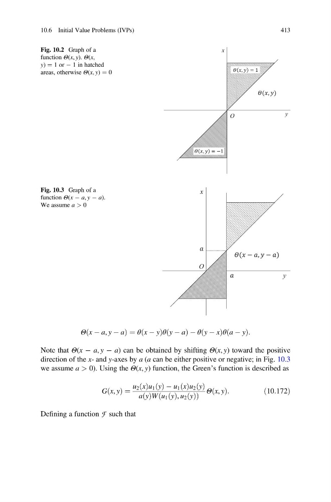
Note that Θ(x À a, y À a) can be obtained by shifting Θ(x, y) toward the positive
direction of the x- and y-axes by a (a can be either positive or negative; in Fig. 10.3
we assume a > 0). Using the Θ(x, y) function, the Green’s function is described as
G x, y
ð Þ ¼
u 2 x
ð Þu 1 y
ð Þ À u 1 x
ð Þu 2 y
ð Þ
a y
ð ÞW u 1 y
ð Þ, u 2 y
ð Þ
ð
Þ
Θ x, y
ð Þ:
ð10:172Þ
Defining a function F such that
x
y
( , )
, = −1
, = 1
O
Fig. 10.2 Graph of a
function Θ(x, y). Θ(x,
y) ¼ 1 or À 1 in hatched
areas, otherwise Θ(x, y) ¼ 0
x
y
( − , − )
O
Fig. 10.3 Graph of a
function Θ(x À a, y À a).
We assume a > 0
10.6 Initial Value Problems (IVPs)
413
ð
Þ¼θ x À y
ð
Þθ y À a
ð
ÞÀθ y À x
ð
Þθ a À y
ð
Þ:
Note that Θ(x À a, y À a) can be obtained by shifting Θ(x, y) toward the positive
direction of the x- and y-axes by a (a can be either positive or negative; in Fig. 10.3
we assume a > 0). Using the Θ(x, y) function, the Green’s function is described as
G x, y
ð Þ ¼
u 2 x
ð Þu 1 y
ð Þ À u 1 x
ð Þu 2 y
ð Þ
a y
ð ÞW u 1 y
ð Þ, u 2 y
ð Þ
ð
Þ
Θ x, y
ð Þ:
ð10:172Þ
Defining a function F such that
x
y
( , )
, = −1
, = 1
O
Fig. 10.2 Graph of a
function Θ(x, y). Θ(x,
y) ¼ 1 or À 1 in hatched
areas, otherwise Θ(x, y) ¼ 0
x
y
( − , − )
O
Fig. 10.3 Graph of a
function Θ(x À a, y À a).
We assume a > 0
10.6 Initial Value Problems (IVPs)
413