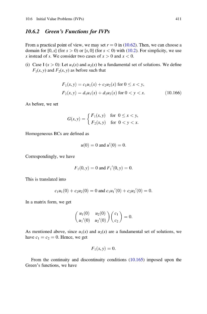
10.6.2 Green’s Functions for IVPs
From a practical point of view, we may set r ¼ 0 in (10.62). Then, we can choose a
domain for [0, s] (for s > 0) or [s, 0] (for s < 0) with (10.2). For simplicity, we use
x instead of s. We consider two cases of x > 0 and x < 0.
(i) Case I (x > 0): Let u 1 (x) and u 2 (x) be a fundamental set of solutions. We define
F 1 (x, y) and F 2 (x, y) as before such that
F 1 x, y
ð Þ ¼ c 1 u 1 x
ð Þ þ c 2 u 2 x
ð Þ for 0 x < y,
F 2 x, y
ð Þ ¼ d 1 u 1 x
ð Þ þ d 2 u 2 x
ð Þ for 0 < y < x:
ð10:166Þ
As before, we set
G x, y
ð Þ ¼
F 1 x, y
ð Þ for 0 x < y,
F 2 x, y
ð Þ for 0 < y < x:
&
Homogeneous BCs are defined as
u 0
ð Þ ¼ 0 and u
0 0
ð Þ ¼ 0:
Correspondingly, we have
F 1 0, y
ð Þ ¼ 0 and F 1
0 0, y
ð Þ ¼ 0:
This is translated into
c 1 u 1 0
ð Þ þ c 2 u 2 0
ð Þ ¼ 0 and c 1 u 1
0 0
ð Þ þ c 2 u 2
0 0
ð Þ ¼ 0:
In a matrix form, we get
u 1 0
ð Þ u 2 0
ð Þ
u 1
0 0
ð Þ u 2
0 0
ð Þ
c 1
c 2
¼ 0:
As mentioned above, since u 1 (x) and u 2 (x) are a fundamental set of solutions, we
have c 1 ¼ c 2 ¼ 0. Hence, we get
F 1 x, y
ð Þ ¼ 0:
From the continuity and discontinuity conditions (10.165) imposed upon the
Green’s functions, we have
10.6 Initial Value Problems (IVPs)
411